Juno Instrument Overview

NASA’s Juno Spacecraft carries a science payload consisting of nine instrument packages to provide unprecedented data on Jupiter’s magnetic environment, its gravitational field, the incredibly dense atmosphere & cloud cover, the interior of the planet and Jupiter’s puzzling aurora.

Juno uses it instruments to look for clues about Jupiter’s formation which will allow scientists to infer details on the solar system’s formation since Jupiter maintained its current state since the early stages of the solar system. Also, the mission sets out to determine whether Jupiter has a solid core, find out how much water is present within the planet’s dense atmosphere, & study winds that can reach more than 600 Kilometers per hour.

Juno is carrying the following scientific instruments that are explained in detail below:

• Gravity Science – GS
• Magnetometer – MAG
• Microwave Radiometer – MWR
• Jupiter Energetic Particle Detector Instrument – JEDI
• Jovian Auroral Distributions Experiment – JADE
• Radio and Plasma Wave Sensor – Waves
• Ultraviolet Spectrograph
• Jovian Infrared Auroral Mapper – JIRAM
• JunoCam

Gravity Science – GS

To reveal the interior structure of Jupiter, Juno makes detailed measurements of the planet’s gravitational field which will point to internal structures that are hidden by the planet’s dense atmosphere.

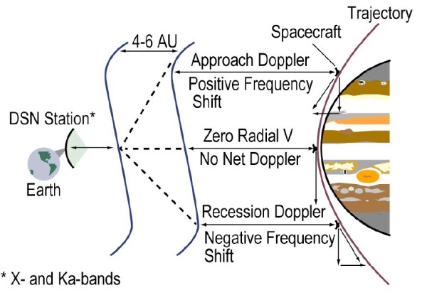
The experiment is a radio science experiment that involves X-Band and Ka-Band ranging from ground stations on Earth to follow the spacecraft in its orbit around the planet and detect even minute changes in the motion of the spacecraft. Local variations in gravity can act on the spacecraft in orbit and cause it to speed up or slow down – those changes in spacecraft motion can be detected using the Doppler Shift in the X and Ka band transponders used by the radio sub-system.

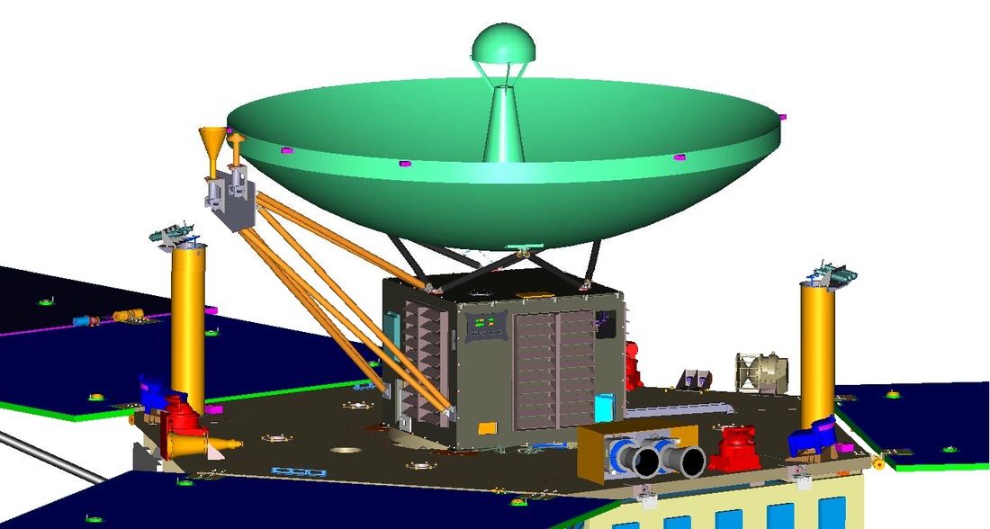
For the gravity experiment, the High Gain Antenna needs to be pointed directly at Earth so that Ka-Band Ranging Signals and X-Band Signals can be sent and received. The Deep Space Network has only one Station capable of providing Ka-Band uplink which is Deep Space Station 25 at DSN Goldstone.

 

Turnaround ranging using the Deep Space Network involves the DSN station that sends an Ka-Band signal to the spacecraft containing ranging tones that it imposes on a carrier using phase modulation. When the spacecraft receives the tones, it sends them right back via X-Band downlink. The DSN station records the timing of the ranging tones uplink and the timing of the tone’s reception order to calculate the line-of-sight distance to the spacecraft.

After processing of the data taking into account delays by the electronics on the spacecraft and the ground, atmospheric and ionospheric properties, interplanetary plasma, and relativistic effects, the ranging method has an accuracy of about one meter in the outer regions of the solar system.

Following corrections for radio signal distortion in Earth’s atmosphere, scientists will be able to use ranging data to map the gravity field of the planet and identify internal features.

 

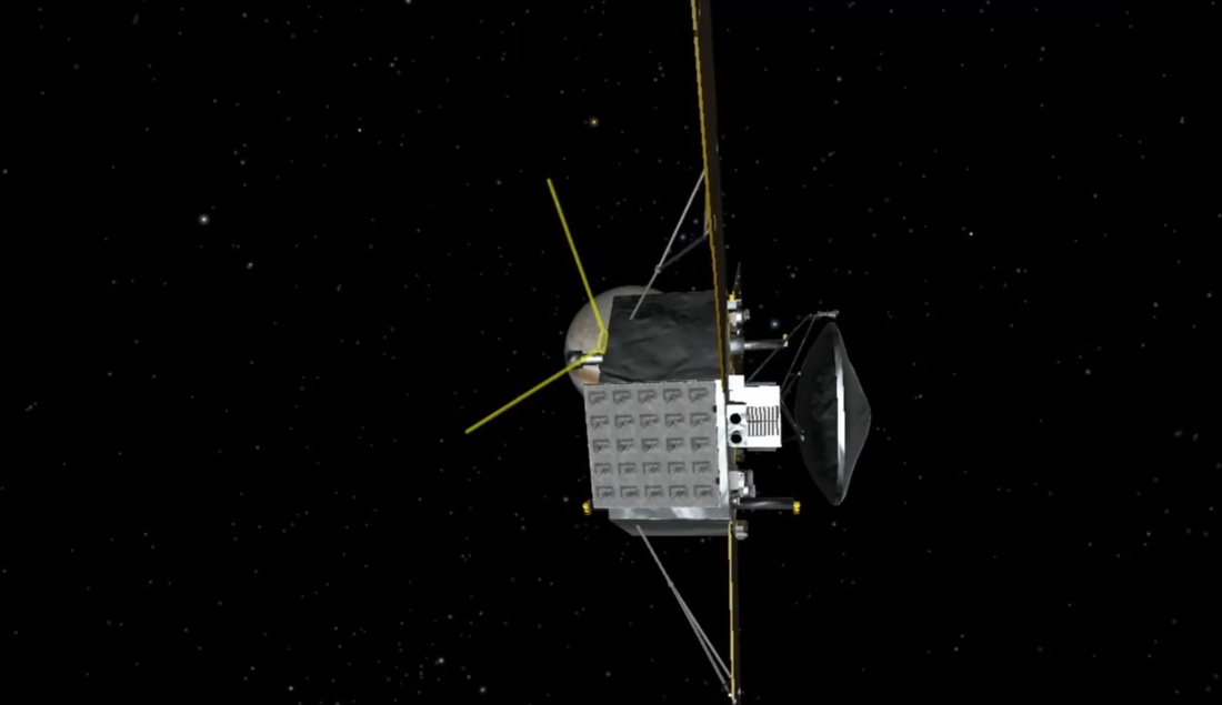
Magnetometer – MAG

 

The MAG instrument of Juno measures Jupiter’s magnetic field to create a detailed three-dimensional map of the Gas Giant’s magnetic environment.

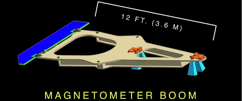
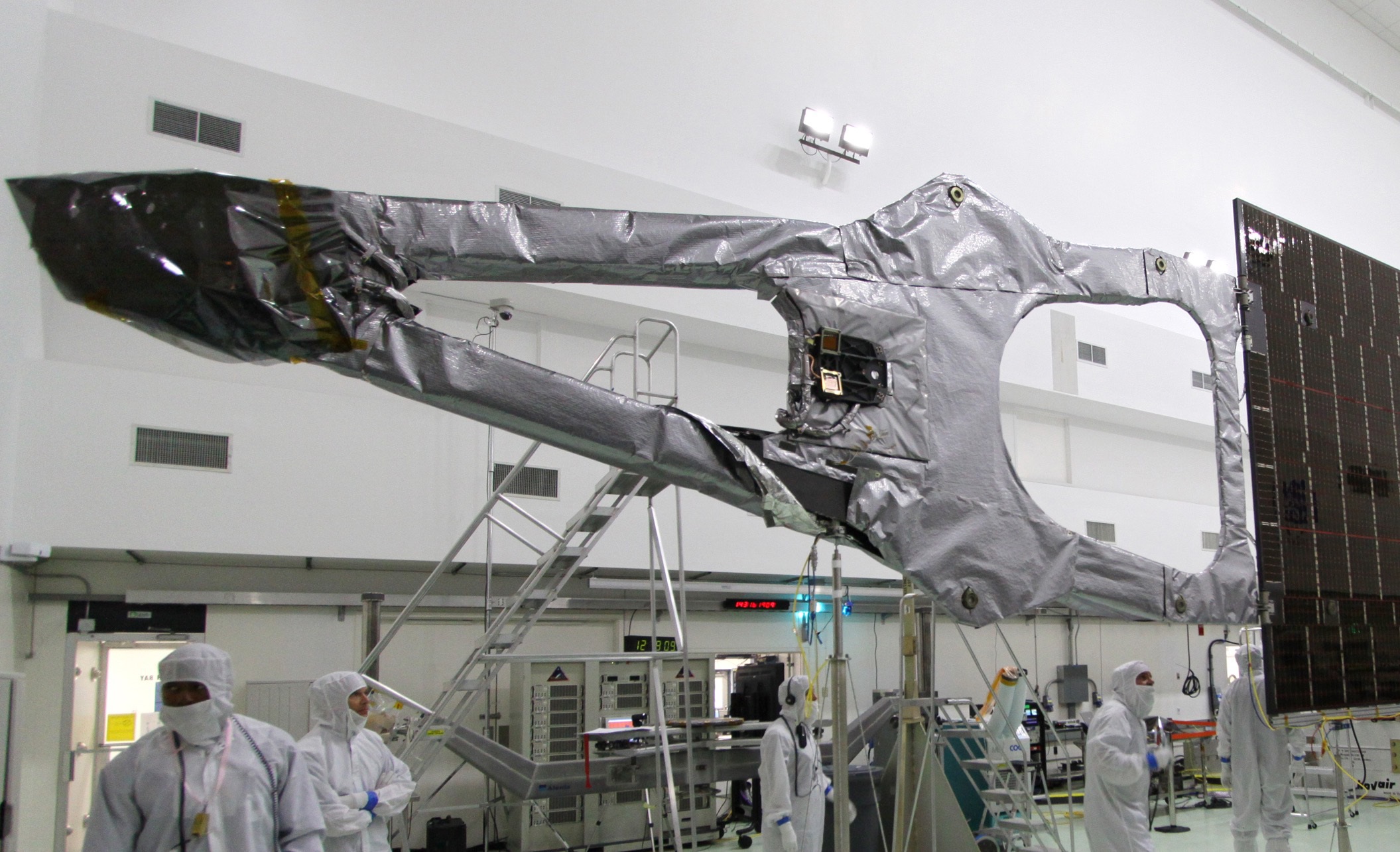
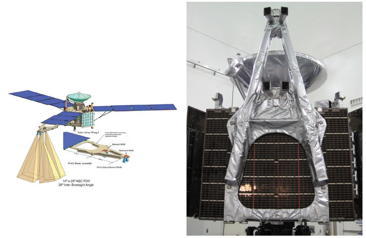
Juno uses a fluxgate magnetometer developed at NASA’s Goddard Spaceflight Center that is installed on one of the three solar arrays of the spacecraft to move the instrument as far away from the spacecraft platform to avoid false readings caused by Juno’s own magnetic emissions.

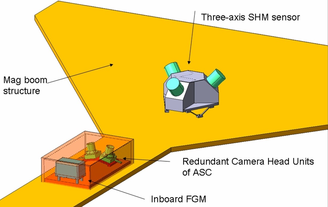
MAG uses dual-fluxgate magnetometers to measure the magnetic field vector and a 3-cell scalar Helium magnetometer sensor provided by JPL is used to measure the strength of the field. An Advanced Stellar Compass provides precise attitude data for each of the sensors.

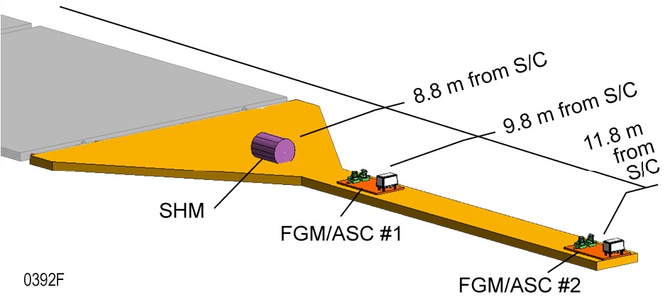
Two fluxgate magnetometers are installed on the magnetometer boom that is installed on the solar array – one is installed 9.8 meters from the spacecraft structure and the other resides 11.8m from the S/C bus and is rotated 180 degrees relative to the other sensor. The scalar Helium magnetometer is located inboard, 8.8m from the platform.

The two fluxgate sensors use the nonlinearity of magnetization properties for the high permeability of easily saturated ferromagnetic alloys to serve as an indicator for the local field strength. The entire Magnetometer instrument weighs 15.25 Kilograms.

 

Having the two fluxgate sensors installed at different distances will allow scientists to determine Juno’s magnetic field that is subtracted from the data to achieve high-precision measurements of Jupiter’s magnetic environment.

“Juno’s magnetometers will measure Jupiter’s magnetic field with extraordinary precision and give us a detailed picture of what the field looks like, both around the planet and deep within,” says Goddard’s Jack Connerney, the mission’s deputy principal investigator and head of the magnetometer team. “This will be the first time we’ve mapped the magnetic field all around Jupiter-it will be the most complete map of its kind ever obtained about any planet with an active dynamo, except, of course, our Earth.”

 

Microwave Radiometer – MWR

The MWR instrument will study the hidden structure beneath Jupiter’s cloud tops – capable of determining on the structure, movement and chemical composition to a pressure of 1,000 atmospheres which corresponds to a depth of 550 Kilometers below the cloud cover. The instrument will help determine the abundance on Water and Ammonia in the Jovian atmosphere.

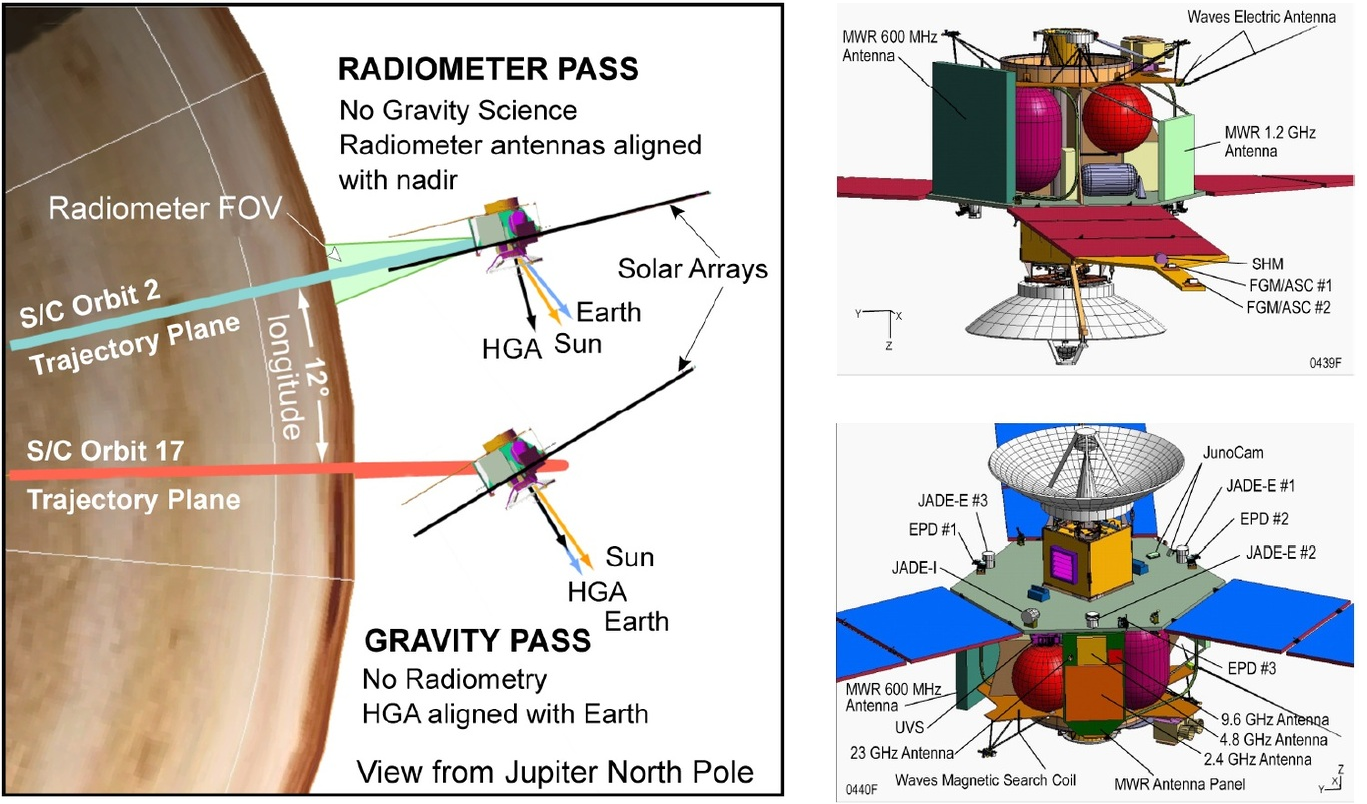
MWR consists of six separate radiometers each with its own antenna and receiver that measure the radiation at six different frequencies along the orbital track of the spacecraft (600 MHz, 1.2 GHz, 2.4 GHz, 4.8 GHz, 9.6 GHz & 22 GHz). The receivers are fed by a combination of patch & slot array antennas as well as horn antennas optimized for the different wavelengths.

 

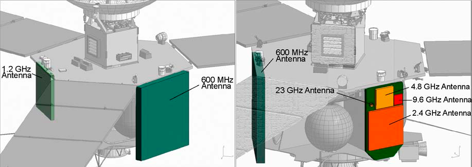
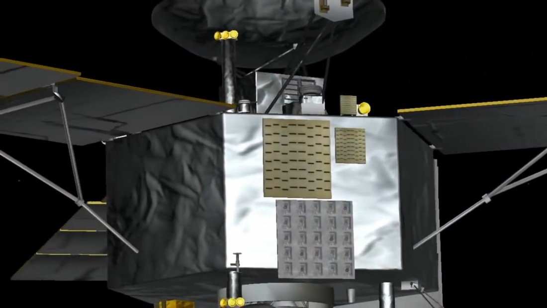
The MWR antennas are mounted on the outside of the Juno spacecraft. The 600 MHz antenna occupies one entire side of the hexagonal spacecraft body and is directly installed on the spacecraft platform. The 1.2, 2.4, 4.8 & 9.6 GHz antennas are installed on a separate support panel attached to another panel on the vehicle’s body. The 22 GHZ antenna is installed on the upper deck of the vehicle. All antennas are connected to the MWR electronics unit via coaxial cables or rectangular waveguides.

The 22 GHz antenna is a profiled corrugated horn with a circular-to-rectangular transition. It is made of solid aluminum and shows a low side lobe performance. The 2.4, 4.8 and 9.6 GHz antennas are waveguide slot array antennas as part of a low-volume, low-mass system. Each antenna has 8×8 slots divided into four 4×4 arrays. The two low-frequency antennas are 5×5 patch array antennas.

The MWR electronics unit has a modular design, consisting of five individual slices: a Power Distribution Unit (2 slices), a Command & Data Handling Unit, and the Housekeeping Unit (2 slices).

The Power Distribution Unit includes six power converters that are connected to the 28-volt spacecraft bus and generate voltages needed by the MWR instrument. The Command & Data Handling Unit includes a 8051 microcontroller based system that processes and executes spacecraft commands and telemetry, controls all data provided by MWR including science & housekeeping data. The system is connected to the main data system of Juno via a redundant RS-422 bus with a transfer rate of 57.6Kb/s. MWR includes a master crystal oscillator to provide precise timing data.

The Housekeeping Units make temperature measurements for radiometric calibrations and they monitor the instrument’s health & bus voltages. A total of 128 multiplexed channels are used to monitor temperature (112 channels) and bus voltages (16 channels). Inside the electronics vault, thermistors are used for temperature measurements while data on the outside of the vehicle is acquired by platinum resistive thermometers that can withstand the extreme radiation environment at Jupiter.

Jupiter Energetic Particle Detector Instrument

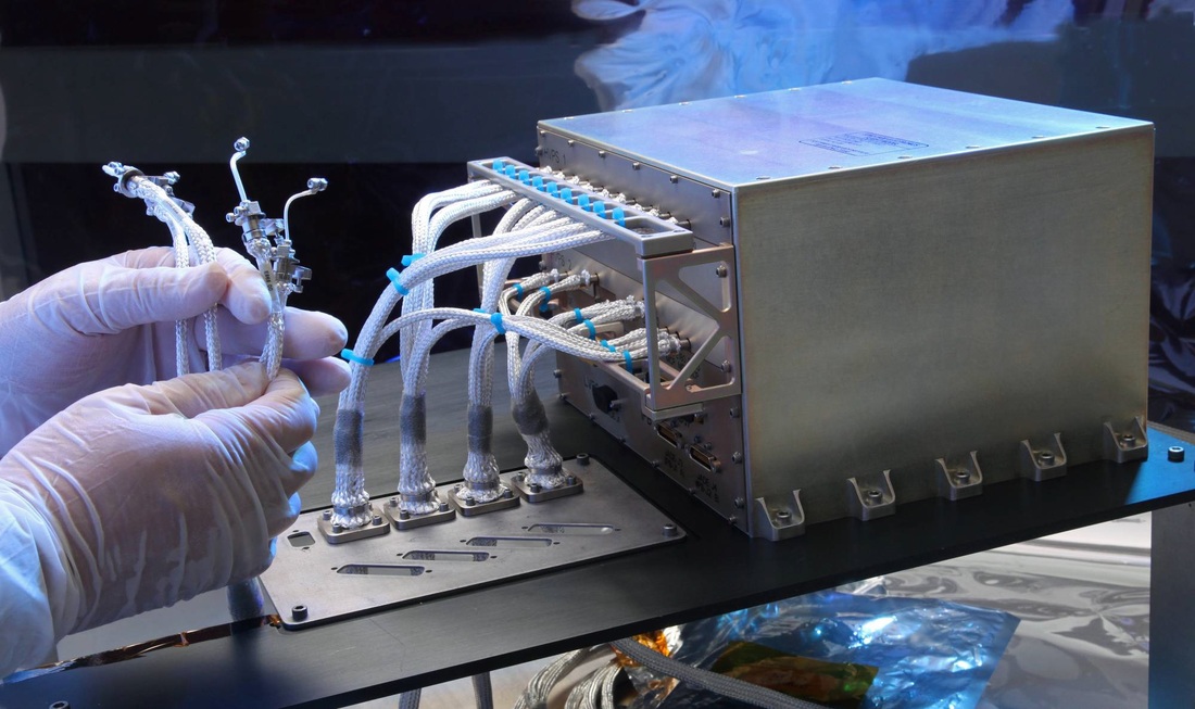
The JEDI instrument will measure energetic particles and their interaction with Jupiter’s magnetic field, investigating Jupiter’s polar space environment with special focus on the physics of the intense Jovian auroras. JEDI measures the energy, spectra, mass species (H, He, O, S), and angular distributions of the higher energy charged particles. The JEDI instrument weighs 6.4 Kilograms including 5 Kilograms of shielding material.

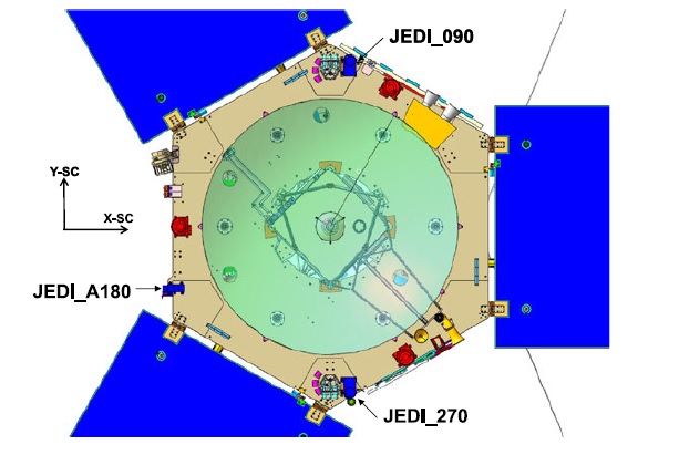
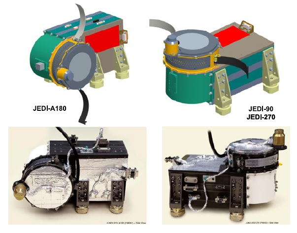
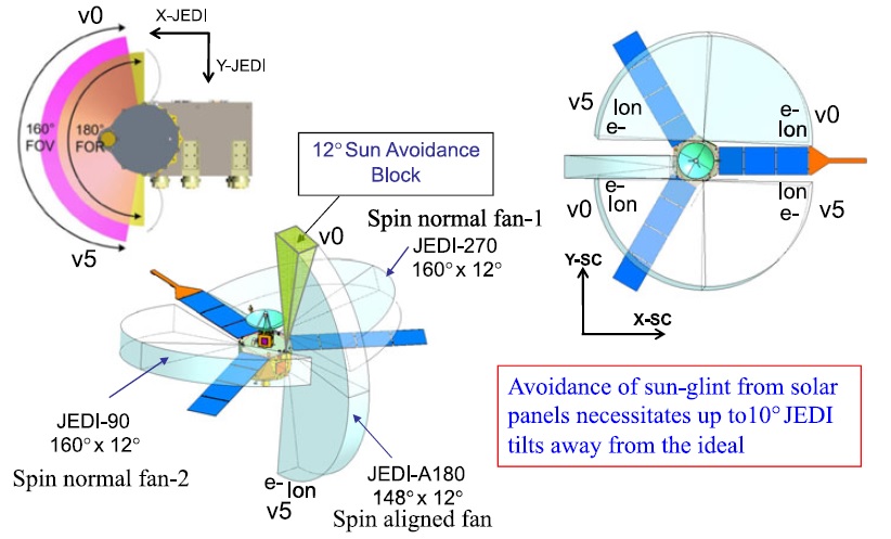
The instrument consists of three nearly identical sensors – each with six ion and six electron views that are arrayed in 12 by 160 degree fans with six 26.7° look directions. Two of those units are installed in a way so that nearly a complete 360-degree coverage normal to the spacecraft spin axis can be achieved in order to get complete pitch angle snapshots. The other sensor is aligned with the spin axis to gather complete sky-views over one spin period of 30 seconds. Each of the JEDI-270/90 units measures 23.3 by 15.9 by 16.1 centimeters while the single JEDI-180 unit is 23.3 by 16.9 by 12.8cm. JEDI sensors are self-contained, they have no additional hardware inside the electronics vault of the spacecraft.

 

Each JEDI Sensor includes the electron and ion sensors as well as detector preamplifiers. The sensor heads and main electronics are integrated as a single unit installed on the Juno spacecraft. The sensor heads have separate data and power interfaces with the spacecraft and run independently of each other.

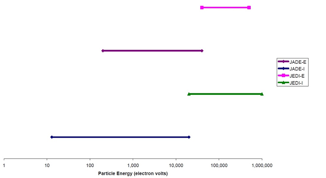
Ions are examined by compact time-of-flight (TOF) by energy and TOF by MCP-Pulse-Height spectrometers that determines three TOF parameters and the energy of ions to identify Hydrogen, Oxygen, Sulfur and other ions. JEDI measures ions at energy ranges of 10keV (kilo electronvolt) to 10 MeV. Electrons from 25 keV to 1 MeV are measured using collimated solid-state detectors that provide energy data and directional distributions.

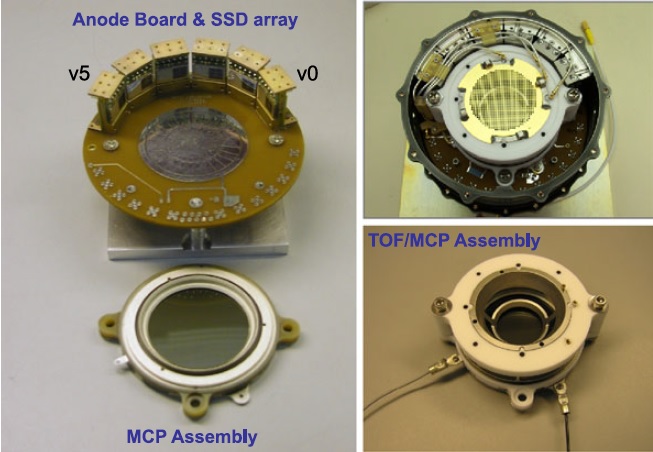
The JEDI sensor heads consist of an aperture opening, electron deflectors, start foils and anodes, a microchannel plate detector, stop anodes and foils, solid state detectors and pre-amplifiers as well as supporting electronics.

The JEDI sensor heads include TOF sections 6 centimeters across that feed the silicon solid-state detectors. The SSD array and the individual pre-amplifiers are connected to an Event Board that determines particle energies.

JEDI Sensor Design

 

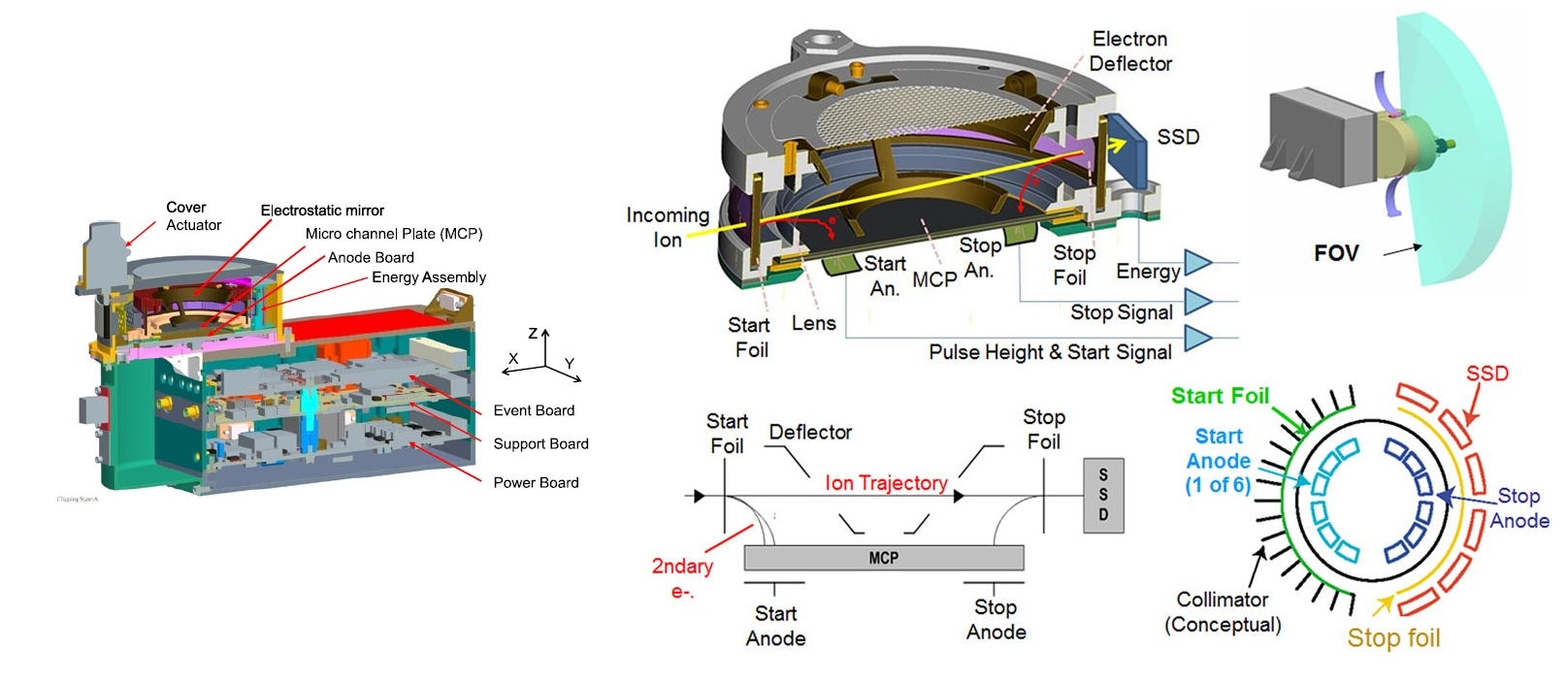
As an ion enters the instrument, it first passes through a thin foil in the collimator (350A Aluminum) before reaching the start foil (carbon-polyamid-carbon) and generating secondary electrons. These electrons are then directed from the primary particle path to the microchannel plate detector where the Start Signal is generated for the Time of Flight measurement. A 500-Volt potential between the foil and the MCP directs the secondary electrons to the TOF detector with high accuracy (1ns dispersion in transit time). The segmented MCP anodes with two start anodes for each of the six angular segments provide data on the direction of travel of the ion.

Secondary electrons that are created as a result of the ion passing through the stop foil are again directed to the MCP and cause a Stop Signal. The time-difference between the two signals represents the time it took the ion to pass through the 6-centimeter TOF instrument.

After the stop foil, ions impact the Solid State Detectors that consist of electron and ion pixels. The SSD determines ion energy which coupled with the TOF measurement delivers ion mass and particle species data. The collimator foil is installed on a high-transmittance grid supported by stainless steel frames. The start/stop foils use a tungsten-copper frame.

Electrons entering the instrument are first decelerated by a 2.6kV potential which is part of the TOF system for ion measurements. 

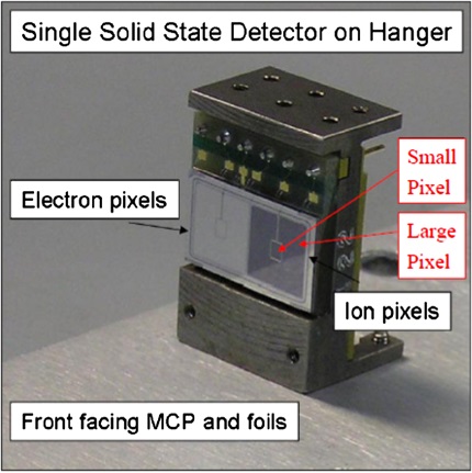
After passing the stop foil, the electrons are again accelerated by a 2.6kV potential. Reaching the SSD detectors, the electrons are detected in the electron pixels that can measure electrons at energies of 25 keV to 1 MeV. The electron detectors are covered with 2-micrometer aluminum metal flashing to reject protons at low energies. Electron measurements do not require a TOF measurement because direction is directly measured by the detector.

The detector system has to be time-multiplexed and can either measure electrons or ions. Three species modes (electron energy, ion energy & ion species, all coupled with direction measurements) are cycled every 0.5 seconds. The six physical SSDs provide a total of 24 SSD pixels (every SSD has 2 electron and two ion pixels – one large pixel of 6.2 by 6.5mm and a small pixel in the center of 1.3 by 1.6mm). Each SSD is connected to a Preamp Board that is part of the sensor assembly.

The electronics box of each sensor holds the event board, power supplies and support electronics. The Event Board interfaces with the sensor to receive TOF signals, SSD data, and MCP pulse heights that are processed by a RTAX2000 16-bit processor. A dedicated Low Voltage Power Supply delivers the low-voltage buses for the various electronics of the sensor while the high-voltage is provided to the sensor head via a High Voltage Supply and Monitor Unit. Data and commands between the instrument and the spacecraft are exchanged via an RS-422 link. Overall, JEDI can process 30,000 events per second.

Each JEDI Sensor head is protected by a cover that is deployed after launch as part of instrument commissioning.

.

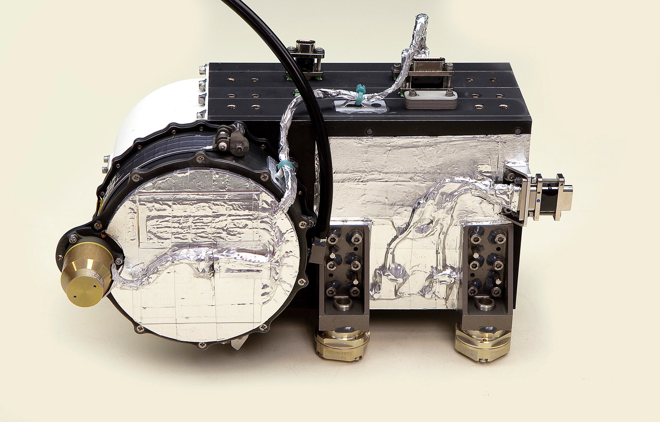
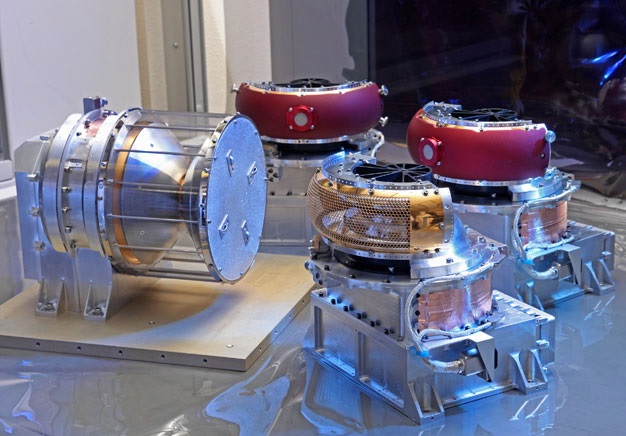
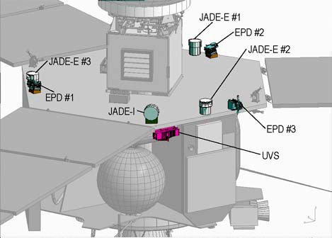
Jovian Auroral Distributions Experiment – JADE

The JADE experiment works with the JEDI and UVS instruments to study the particles and processes that form Jupiter’s powerful auroras.

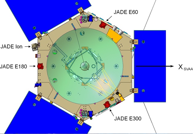
JADE features four deck-mounted sensor packages – three electron analyzers with a field of view of 360 by 90 degrees and a single ion mass spectrometer with a field of view of 270 by 90 degrees. The JADE electronics box that contains all instrument electronics except pre-amplifiers resides inside the electronics vault.

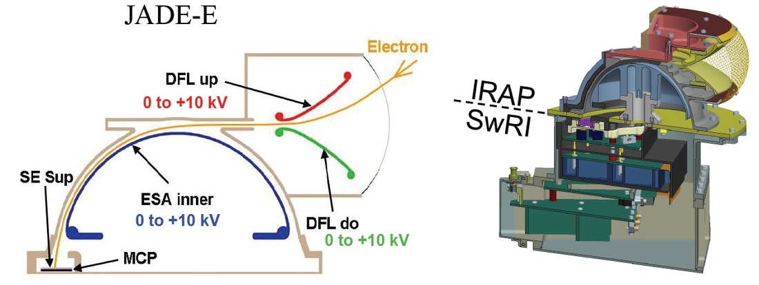
Each electron sensor weighs 5.25 Kilograms and is 21 by 21 by 21 centimeters in size covering an energy range of 0.1 to 95 keV. Each sensor has a field of view of 120 degrees so that a complete 360-degree coverage is achieved. The JADE-E sensors consists of a top-hat electrostatic analyzer, two deflectors and a Multichannel plate detector with an anode ring underneath. Two deflectors, one upper and one lower, change the path of electrons by up to 35 degrees based on their energy before the electrons reach the electrostatic analyzer.

The azimuth angle of impinging electrons is determined by measuring the position in which the electrons impact the MCP detector with a position-sensitive anode while the elevation angle is measured perpendicular to the imaging plane to determine the direction of incoming electrons.

The JADE-E ceramic anode board collects the charge from the MCPs. It is divided into seventeen 7.5-degree segments – 16 of those achieve the 120-degree active field of view while the 17th is providing dark measurements for data processing.

 

Part of the JADE-E electronics suite is a Capacitor Board that decouples the high voltage signals from the anode board to ground potential for processing by the analog electronics of the instrument. The board includes seventeen 1,000pF high voltage (6,000V) capacitors.

The signals are then transmitted to the Charge Amplifier Board that features 17 Amptek charge amplifiers that process the individual MCP pulses to generate a digital output. Next, the Digital Board uses the pulses provided by the 17 A121 amplifiers. Passive termination is utilized to translate the 5V level outputs to the serializer input level of 3.3V.

The serializer transmits the signals via high-speed, low-voltage differential signal lines to the Sensor Interface Board which counts all pulses for all channels at a frequency of 5.55 MHz for each pixel. A High Voltage Distribution Board conditions the incoming high voltage – providing shielded, mechanical termination of the high-voltage coaxial cables, it filters the detector bias signals and sets the proper optical voltage in the detector.

 

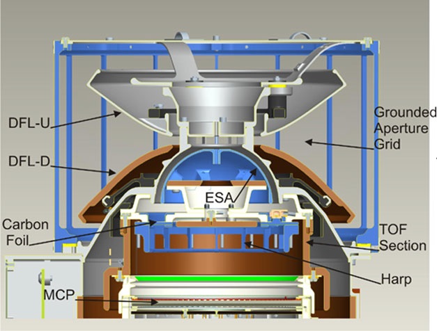
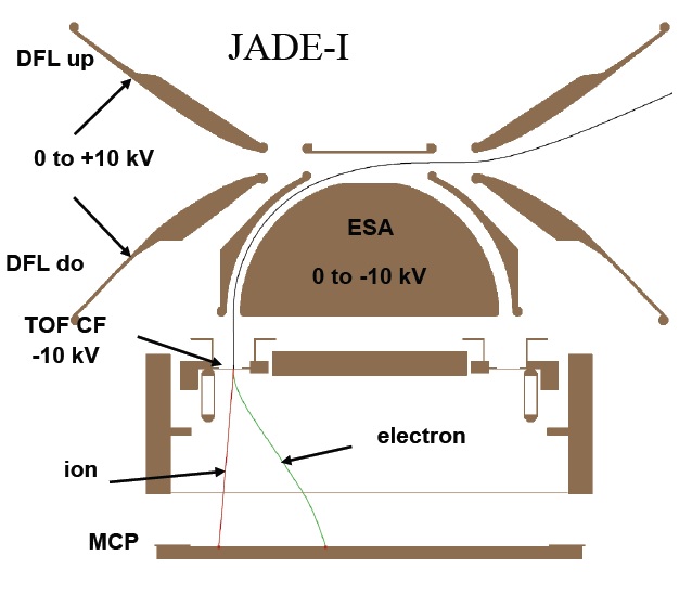
The JADE ion sensor is a spherical top hat electrostatic analyzer that measures ions with an energy range of 10eV/q to 45eV/q for ion masses from 1 to 40 atomic mass units. The sensor’s field of view has a plane offset of 15 degrees from the spacecraft x-axis. Incoming ions first pass two deflectors that sweep the look direction to to 45 degrees before passing through a 90-degree spherical section electrostatic analyzer to select the energy per charge of positive ions. To reduce noise created by UV radiation, the sensor uses nickel-plated titanium inside the analyzer dome and a grounded grid that is covering the entire sensor with an effective transmission of 86%.

When entering the Time of Flight section of the instrument, ions are accelerated by 10keV. Secondary electrons are generated when an ion passes through an ultra-thin carbon foil – these electrons are accelerated to 8keV and are detected in a dedicated position on the Multichannel plate detector. When the electrons are detected, a start signal is transmitted and when the ion arrives, a stop pulse is generated to determine Time of Flight. The ion is detected on one of 12 anodes that are installed next to each other to provide ion elevation data with a sufficient resolution. JADE-I weighs 7.55 Kilograms and is 18 by 24 by 22 centimeters in size consuming two watts of power.

Similar to JADE-E, the JADE-I electronics consist of five separate boards. Its ceramic anode board contains a start anode in the center that provides the signals of the MCP that collects the start-electrons which are emitted as ions pass the carbon foil. The outer ring is divided into thirteen 22.5-degree anode bins – 12 of which form the 270 -degree field of view with a single dark-measurement channel. The 12 anode bins are used to generate the stop signal to measure Time of Flight and they provide the elevation of incoming ions.

For TOF determination, a dedicated TOF board is used that receives the signals from the start anode and the sum of all anode signals that is provided by the amplifier board. The TOF board converts those signals to digital start and stop pulses that are passed along to the E-box. The minimum pulse-pair resolution is 1.45 nanoseconds while the longest allowed TOF is 330ns. The JADE-I Charge Amplifier Board is similar to that used on JADE-E – just with a different number and arrangement of the A121 units to match the position of the 13 anodes on their board. It provides the input from each stop anode to a summing amplifier for relay to the TOF board while each separate channel output is also sent to the Digital Board which is also similar to the JADE-E DB.

It registers the pulses from the 13 A121 outputs and translates them for the serializer for signal transmission to the E-box. JADE-I also has its own High Voltage Distribution Board.

The JADE E-box is installed in the Radiation Vault of Juno and contains within it a Low-Voltage Power Supply Module, an Instrument Processing Board, the Sensor Interface Board and two High-Voltage Power Supplies.

The JADE flight software runs on the Instrument Processor Board that provides instrument control and command actuation using a cPCI master bus. The IPB executes spacecraft commands, transmits low-rate science and housekeeping data as well as high-rate Burst Mode Science data in data packets that are formatted by the IPB before being sent to the Juno data system. It uses a 128KB EEPROM for the core boot code, a 512KB EEPROM to hold copies of its flight software and data tables, and a 4GB SRAM for code and data when the flight software is executing.

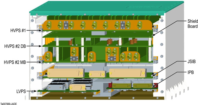
The Low-Voltage Power Supply is connected to the two redundant 28-Volt main buses and provides the JADE voltages of 3.3, +/-5 and +/-12 Volts. The High-Voltage Power Supply generates the high-voltages required for JADE-E and I. The first HVPS board provides a +10.5kV power supply for each of the three JADE-E sensors. Linear regulators generate the 10V to 10kV stepping supplies for the two deflectors and the electrostatic analyzer. The second board generates high voltages for the programmable Multi-channel Plate power supplies – three +3.8kV supplies for the JADE-E and one -3.8kV for the JADE-I MCP as well as a -10kV TOF power supply.

The JADE Sensor Interface Board commands all high-voltage power supplies, processes raw count data from all events on all sensors, and determines the coincidence in the JADE-I sensor. Anode counts from each sensor are de-serialized and recorded in histograms or real-time count-rate registers.
TOF data is generated by a Time-to-Digital converter. Also, test pulses can be used by the JSIB to check all the amplifiers used in the individual instruments. JSIB also measures 80 housekeeping telemetry parameters that can be stored and read-out by the IPB for downlink to the ground to provide insight into instrument health.

The JADE backplane connects all the different electronics modules using PCI interfaces.

JADE & JEDI Coverage

 

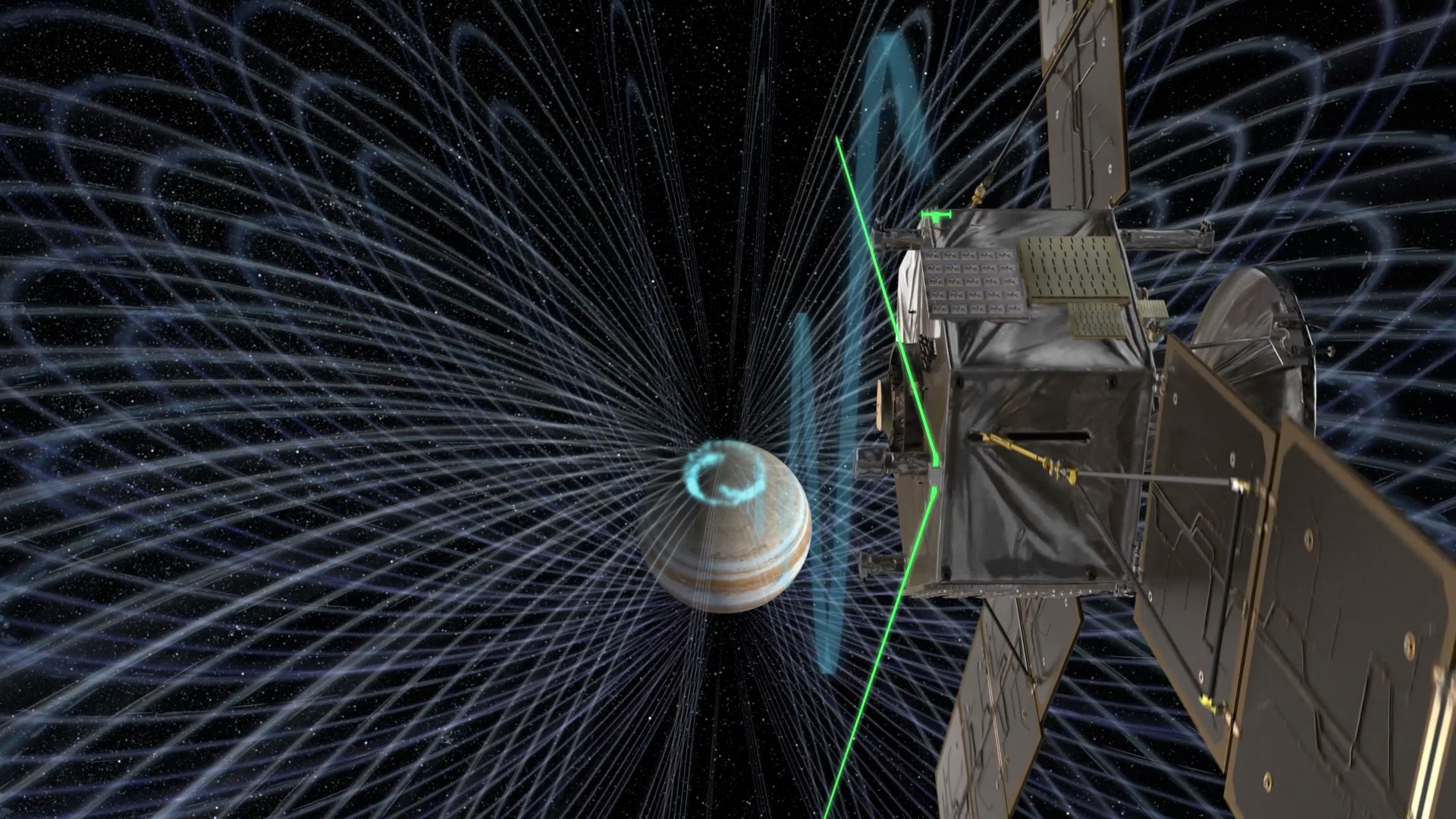
Radio and Plasma Wave Sensor – Waves

The Waves instrument measures radio and plasma waves in the Jovian magnetosphere to help understand interactions between Jupiter’s magnetic field, the magnetosphere and the atmosphere. It measures the electric and magnetic field components of in-situ plasma waves and freely propagating radio waves.

The instrument consists of a V-shaped antenna that measures four meters from tip to tip – a dipole antenna to measure electric fields, and a magnetic search coil to measure the magnetic component. Waves electronics are installed inside the Radiation Vault.

The dipole antenna and its electronics are built to analyze electric fields in the frequency range of 50Hz to 40MHz. The antenna consists of two elements each 2.8m in length. These elements are extended in a plane rotated 45 degrees to the aft of the aft deck with a subtended angle of 120 degrees. The antenna is installed aft of the solar panel wing that features the Magnetometer Boom to be symmetric with the wing.

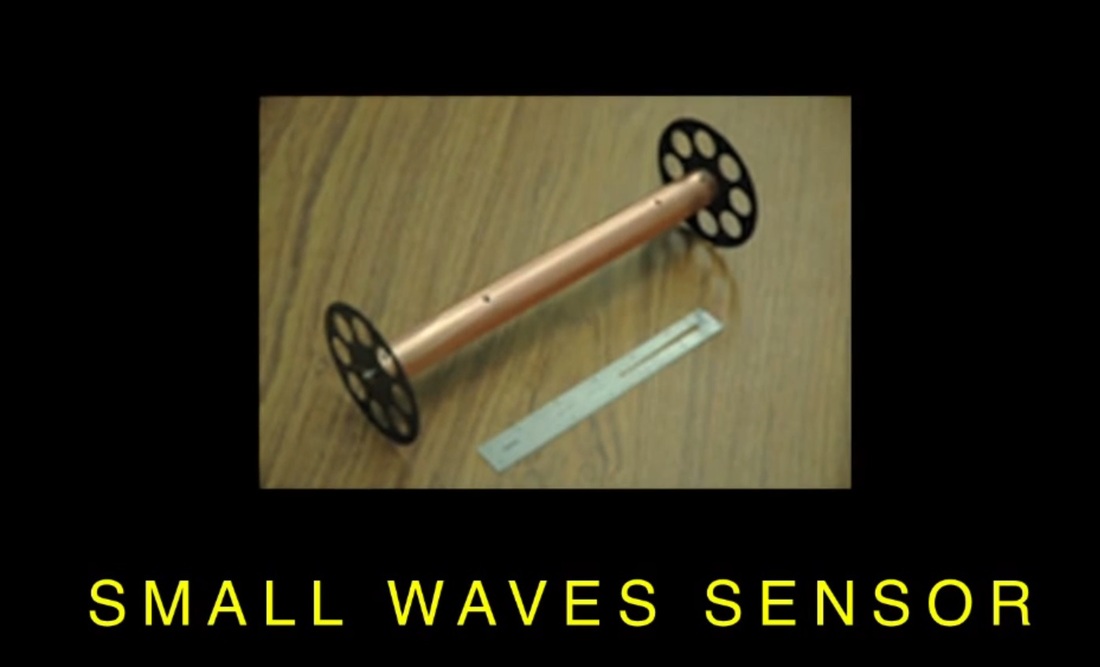
The magnetic search coil consists of a fine copper wire wrapped 10,000 times around a 15-centimeter mu-metal core (77% nickel, 16% iron, 5% copper 2% chromium) – an alloy that has a very high magnetic permeability. The search coil is installed on the aft flight deck parallel to the spacecraft z-axis which itself is parallel to the spacecraft spin axis. This is done to minimize the effects of the very strong magnetic field of Jupiter rotating as the vehicle spins at 2rpm near perijove. The magnetic search coil measures wave magnetic fields from 50hz to 20kHz.

The Waves sensor electronics consist of two receivers – a low and a high frequency receiver. The low frequency receiver includes two channels that are covering the frequency range of 50 Hz to 20 kHz. The system operates in two configurations – one allows for simultaneous sampling of electric and magnetic sensor data and the other configuration uses a signal from the Juno Power Distribution Unit to reflect voltage fluctuations on the bus to be used in a noise cancelling mode with either the electric or the magnetic signal being analyzed in the second channel. The third channel of the Low Frequency Receiver is a high band that covers frequencies of 10 kHz to 150 kHz used for electric signals only with noise cancelation capability.

The High-Frequency Receiver is comprised of two nearly identical units – one used to analyze data from 100 kHz to 40 MHz and the other allows for high-resolution waveform measurements in a 1-MHz band.

 

The baseband receiver includes a variable gain amplifier, a 100 kHz to 3 MHz bandpass filter and a 12-bit analog-to-digital converter. The second receiver is a double sideband heterodyne receiver detecting the amplitude of signals in 1-MHz bandwidths from 3 to 40 MHz as a swept frequency receiver.

The Waves Data Processing Unit consists of two field programmable gate arrays.

The first is responsible for Waves instrument operations including command execution, data output functions, observation scheduling and onboard analysis. The second FPGA is optimized to carry out Fourier transforms and other signal processing operations to move signal analyses from the analog to the digital domain – performing spectrum analysis, spectral binning and averaging, and noise cancelation.

Ultraviolet Spectrograph

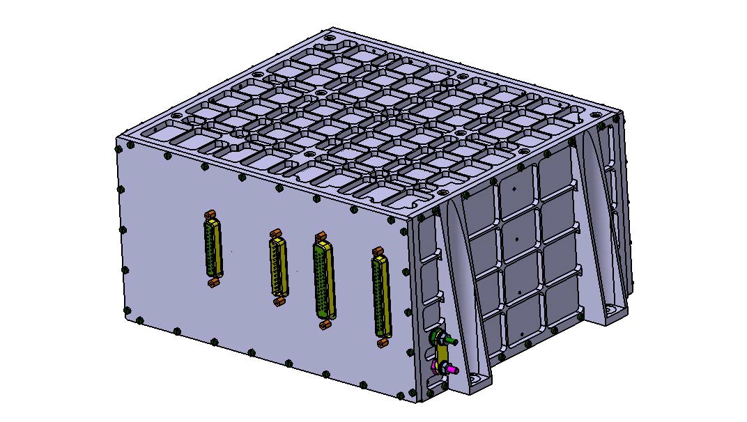
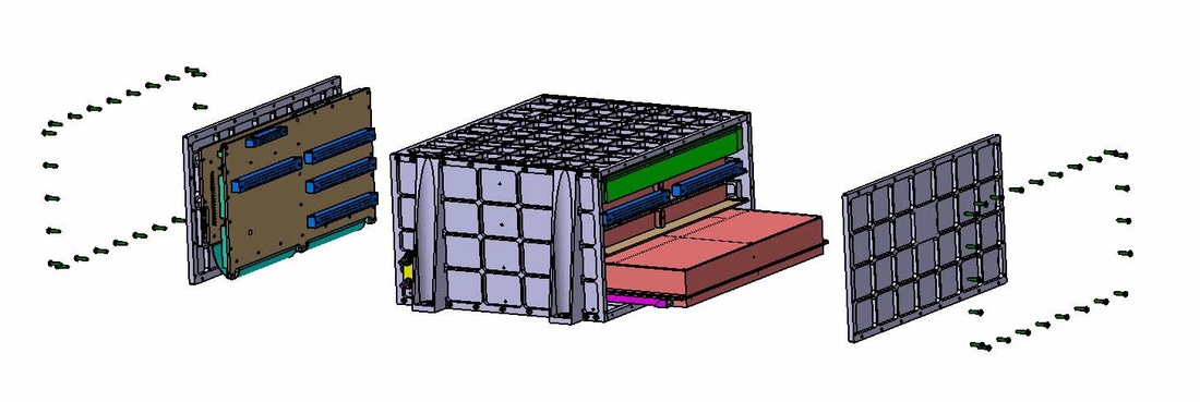
Juno’s Ultraviolet Spectrograph Payload, UVS for short, images and measures the spectrum of the Jovian aurora in the 70 to 205-nanometer range of the electromagnetic spectrum. UVS data will be used to characterize and investigate the sources of Jupiter’s powerful auroras. The instrument consists of two components – the dedicated optical assembly and the instrument electronics box that resides within the radiation vault of the spacecraft.

Overall, the instrument weighs about 21.5 Kilograms and consumes 9 Watts of electrical power.

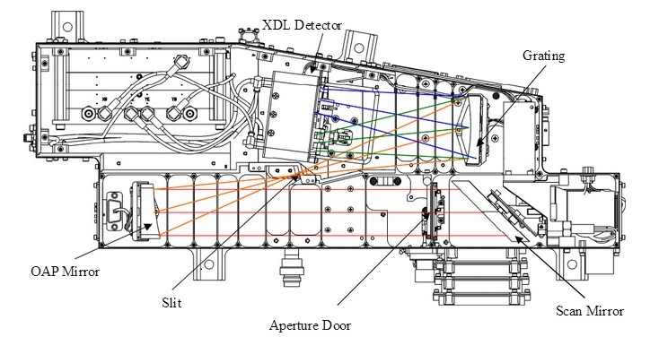
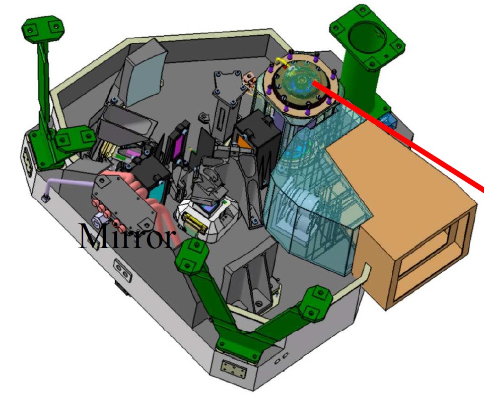
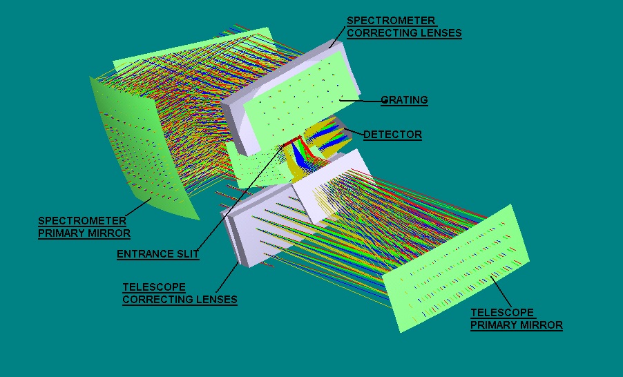
The telescope/spectrograph assembly is installed on the Juno instrument deck viewing radially outward from the spinning spacecraft in order to scan an area of Jupiter. The telescope of the instrument feeds a 0.15-m Rowland circle spectrograph. Light enters the UVS telescope via a flat scan mirror and passes through an input aperture of 40 by 40 millimeters. The scan mirror is used to target specific auroral features by moving the mirror up to +/-30 degrees perpendicular to the Juno spin axis. The light is collected and focused by an off-axis parabolic primary mirror with a focal length of 120 millimeters. The scan and primary mirrors are coated with aluminum and an overcoat of magnesium fluoride which maximizes the reflection at wavelengths longer than 100nm.

The UVS spectrograph entrance slit uses a dog-bone structure, being 6° long with three 2-degree sections of 0.2°, 0.5° and 0.2° width creating a field of view of 0.05° in the dispersion direction and 2° in the spatial direction in the center of the field of view. In between the sections of the dog-bone slit are bars of material to reduce stray light. This slit design with a thin center section and wide edges realizes a maximum resolution and throughput while reducing stray light.

 

Light entering the entrance slit is dispersed by a toroidal holographical grating with 1600 grooves per millimeter and a Rowland circle diameter of 150mm. The grating also uses the reflective magnesium fluoride coating. The dispersed light is then passed to the detector assembly.

UVS uses a microchannel plate (MCP) cross delay line (XDL) detector with a solar blind UV- sensitive CsI photocathode. The CsI photocathode covers a spectral range of 67.5 to 210 nm. The MCP detector uses the 2048 by 256 pixel format and is cylindrically curved to match the Rowland circle in order to optimize the spectral and spatial focus of the instrument. The detector assembly is shielded by Tantalum panels that protect the detector and the adjacent detector electronics from high-energy electrons in the MeV energy range. All optical components of the UVS instrument are installed on aluminum structures to minimize thermal defocus effects.

The main electronics box of UVS located inside the electronics vault includes two redundant high-voltage power supplies (HVPS) that supply the high-operating voltage to the MCP, two redundant low-voltage power supplies provide power to the instrument electronics, the command and data handling (C&DH) electronics, heater/actuator activation electronics, scan mirror electronics, and event processing electronics. The UVS controller uses an Actel 8051 microcontroller. UVS operates at detector count rates of up to 83kHz using a pixel list data collection mode.

UVS achieves a spectral resolution of 0.4 to 0.6 nanometers in point-source operation and 1 to 1.2 nm in extended source operation. The instrument has a spatial resolution of 0.1 degrees, equivalent to 125 Kilometers at a distance of 1 Jupiter radius. The instrument field of regard is 360° (full revolution of the spacecraft) by 60° (+/-30° scan mirror motion).

Jovian Infrared Auroral Mapper – JIRAM

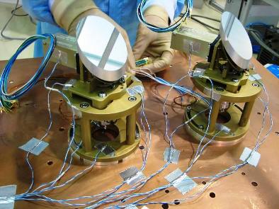
The JIRAM instrument combines an infrared imager and spectrometer to obtain high resolution images of Jupiter’s atmosphere and auroral display in the 2 to 5 micrometer range. JIRAM data contributes to studies of the polar aurora and atmospheric dynamics through complementary measurements using the other instruments. The instrument’s optical head and electronics are hosted on the instrument deck of the spacecraft. Overall, JIRAM weighs about 8 Kilograms and has a peak power consumption of 16.7 Watts.

Covering the spectral range of 2 to 5 micrometers allows JIRAM to observe the absorption maxima of water at 2.7 and 2.9 µm and methane around 2.3 and 3 µm. JIRAM will be able to study the Jovian atmosphere between 0.2 and 3 to 10 bar depending on its composition. Using the 4-5 µm band, JIRAM can observe clouds in the upper regions of Jupiter’s dense atmosphere as well as auroral emissions at 3.4 µm and Hot Spots at the upper end of JIRAM’s range at 5 µm.

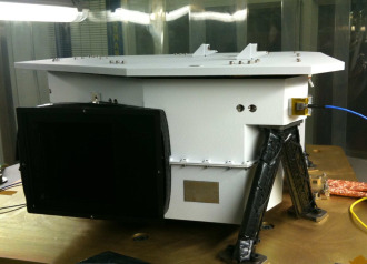
The JRIAM instrument uses a single telescope that facilitates both an infrared camera and a spectrometer to realize a large observational flexibility. The JIRAM assembly is installed on the instrument deck using three bipods. Thermal control is accomplished by a primary and a secondary radiator.

 

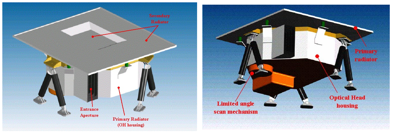
The 47-millimeter JIRAM Entrance Aperture points radially outward to see Jupiter underneath as the spacecraft spins in its orbit. Light that enters the aperture is passed onto a De-Spin mirror that can be moved in the along-track direction to remove the spin of the spacecraft to facilitate the readout time of the JIRAM detector in order to create one image/one slit every 2.5 seconds and ensure continuous coverage. The De-Spin Mirror is controlled by the instrument controller that commands the De-Spin Mirror Driving Board which actuates the motor that holds the mirror assembly.

Next, the light enters the telescope that uses two dioptric doublets to correct aberrations. The telescope has a field of view of 13.7 by 13.7 degrees. After passing through the telescope, the focused light is passed onto a beam splitter that creates two optical paths with two focal planes that are located at the focal point of the telescope.

The beam that is transmitted by the beam splitter enters Focal Plane Assembly #1 which is responsible for optical imaging using two bandpass filters in the L-Band at 3.3 to 3.6 micrometers and the M-Band at 4.55 to 5.05 micrometers. Images using the M- and L-Band filters can be taken at the same time. (As the spacecraft moves, the observed area is first seen by the M-Band portion followed by the L-Band portion of the imager.) Each detector is a HgCdTe CMOS Detector with a size of 432 by 128 pixels with pixel sizes of 38 by 38 micrometers. The infrared imager has a field of view of 3.66 by 6.24 degrees.

 

In the focal point of the reflected beam is the spectrometer entrance slit. The JIRAM spectrometer uses a Littrow design. The incoming light is passed onto a primary mirror that directs the light to the spectrometer optics. The collimated light then passes to a diffraction grating that is 60 by 32 millimeters in size and has 30.2 grooves per millimeter. The grating has a high efficiency of 90% with low stray light values. Another set of optics focuses the diffracted light onto the spectrometer detector. The detector is 256 by 336 pixels creating a spectral resolution of 9 nanometers in the spectral range of 2.0 to 5.0 micrometers. The spectrometer has a field of view of 3.5 degrees across track by 50 arcsec along track which creates a spatial resolution at the 1 bar level that varies from 1 to 200 Kilometers as a function of orbital altitude.

The infrared imager and spectrometer operate simultaneously to create two-dimensional spectral images of the same area on Jupiter.

 

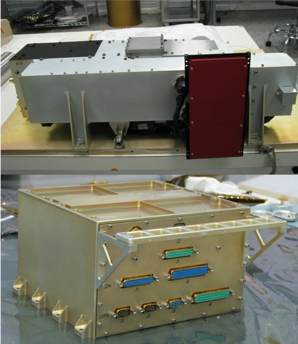
The electronics box of the JIRAM instrument measures 24.4 by 21.3 by 13.5 centimeters and is also installed on the Juno instrument deck. The box houses the Proximity Electronics Board, the instrument controller, the mirror motor board and power supply electronics. The instrument controller is connected to the spacecraft Command/Data Handling system via an RS-422 bus. JIRAM sends science data and telemetry to the spacecraft and receives commands for instrument operations and timing synchronization data from the spacecraft.

The instrument controller regulates all functions of the instrument, controlling the observation sequences and commanding the various electronics boards.

The Proximity Electronics Board provides actuation of the focal plane assembly, the mechanical shutter of the instrument, the main heaters of the optical head and the calibration lamp that is used for instrument calibration and performance monitoring. The PEB is also in charge of instrument read-out and data transfer.

The De-Spinning Motor Board drives the De-Spin mirror based on commands from the instrument controller. Instrument power is provided via a DC/DC conversion board, survival heaters are connected directly to the 28-Volt spacecraft bus.

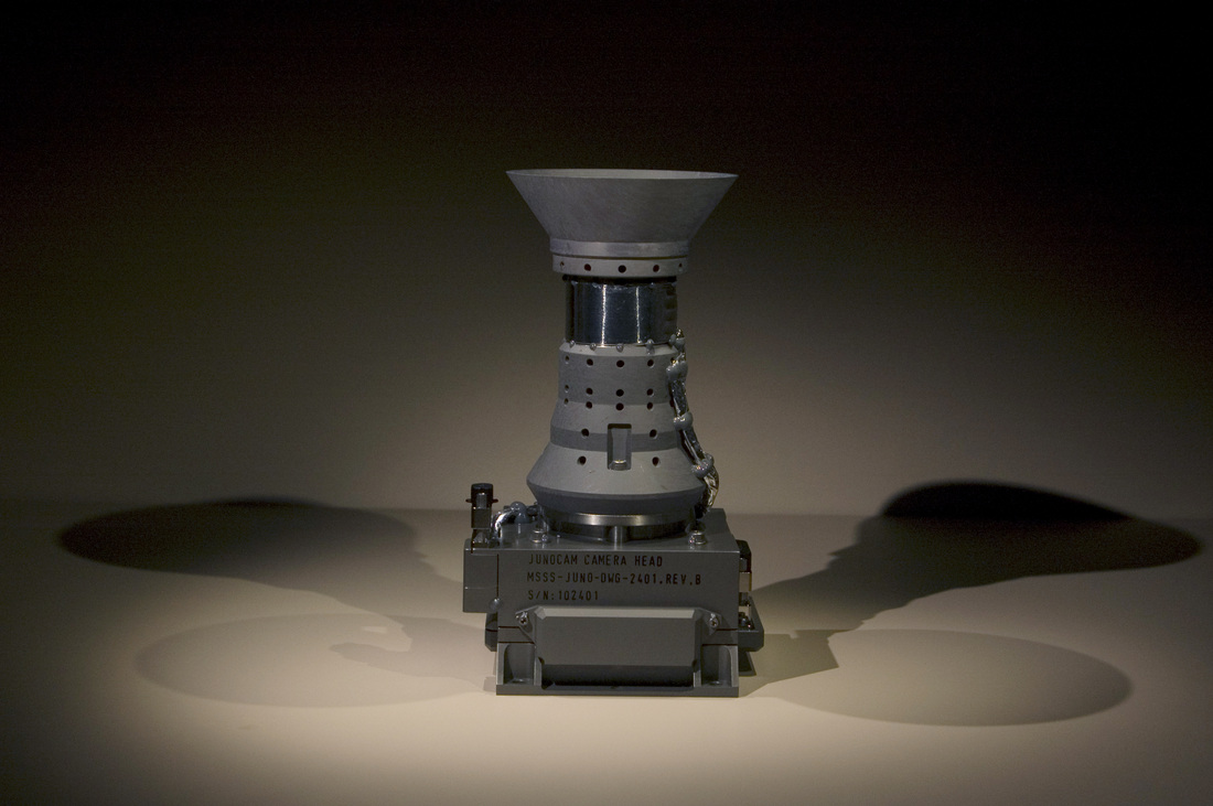
JunoCam

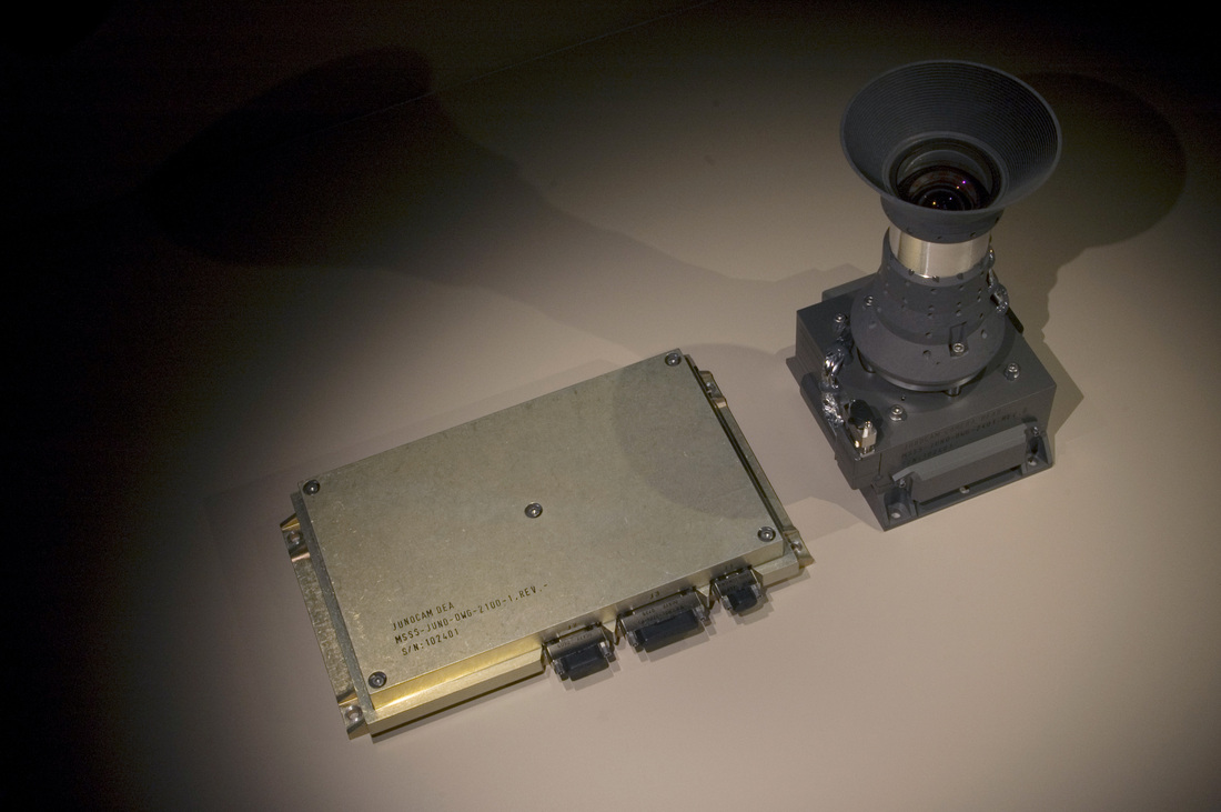
JunoCam is a visible spectrum camera to deliver full-color images of the Jovian atmosphere at medium resolutions. The instrument will be used for education and public outreach and scientific studies conducted by students. The instrument was provided by Malin Space Science Systems and is based on the Mars Descent Imager flown on the Curiosity rover.

JunoCam consists of two parts, both installed outside of the radiation vault, the camera head that includes the optics assembly, detector, the front-end detector electronics, and the JunoCam electronics box that houses the instrument electronics, the image data buffer and power supplies.

The JunoCam instrument is a pushframe imager using the 2RPM spin rate of the Juno spacecraft to build its image, using Time Delay Integration. The camera has a field of view that is about 58 degrees across and can achieve 360-degree coverage as Juno completes one revolution. JunoCam uses a 1600 by 1200-pixel CMOS detector (11.84 x 8.88mm, pixel size 7.4 µm) using four filters – the standard RGB filter to create full color images using blue (420-520nm), green (500-600nm) and red/IR (600-800nm) filters. The RGB field of view is 4.64 by 58 degrees. The fourth wavelength band imaged by JunoCam is the methane band at 890nm to study the abundance of methane in the Jovian atmosphere. The methane band covers a field of view of 10.2 by 58 degrees. Typical exposure times for JunoCam will vary from 0.5 seconds in the methane band to 12.5 microseconds for the visible bands. JunoCam has a focal length of 11.7mm.

When passing perijove, JunoCam is capable of creating images with a resolution of 15 Kilometers per pixel to provide close-up views of the Jovian atmosphere and possible auroral displays. When Juno flies over the poles, Jupiter will roughly fill the field-of view of JunoCam. At apojove, Jupiter will only be 75 pixels in size, thus JunoCam will be most active when Juno is close to Jupiter. Imaging the moons of Jupiter is also not feasible due to the small size of the moons and the great distance of the spacecraft to them.

Over the course of one orbit, Juno will be limited to a data downlink of 40 MB of JunoCam images. The photos will be stored in raw data formats however, real time compression (lossless and lossy JPEG) is available. Depending on the compression, 10 to 1000 photos will be downlinked per orbit. Due to the harsh radiation environment around Jupiter, JunoCam is expected to remain operational for the first seven orbits of the mission, however, teams hope to operate the camera longer than that if possible.