Magnetospheric Multiscale Mission

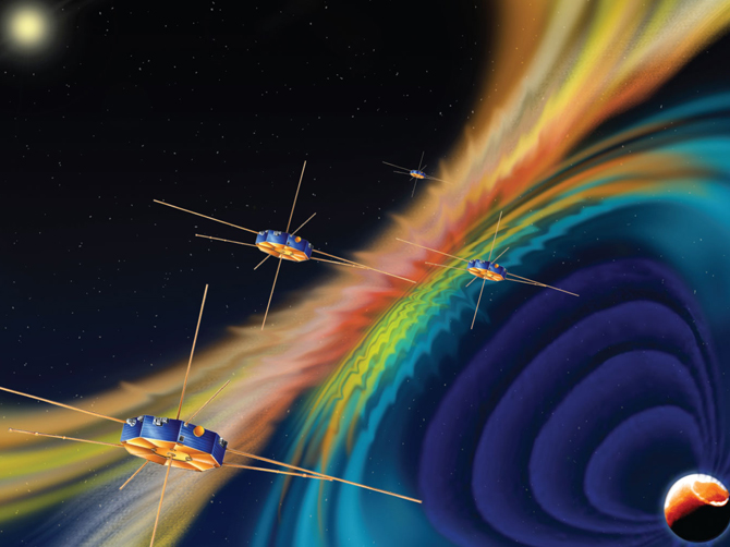
The Magnetospheric Multiscale Mission or MMS is a NASA solar-terrestrial science mission consisting of four identical spin-stabilized spacecraft outfitted with instrumentation to measure plasmas, fields and particles to study processes ongoing in Earth’s magnetosphere. Flying in a precise formation, the four spacecraft will be able to separate local and time-dependent variability and make measurements at unprecedented temporal resolution to shed light on a number of processes ongoing in the magnetosphere and magnetospheric interaction with the sun’s magnetic field.

MMS aims to study the microphysics of three fundamental plasma processes that occur in the magnetosphere: magnetic reconnection, particle acceleration and turbulence – processes that are common in all astrophysical plasma systems underlining the importance of these measurements for a better understanding of such systems. For Earth, these processes play a major role in space weather phenomena that can have an effect on satellites in orbit as well as power grids on Earth. MMS will study magnetospheric properties on scales of a few tens of Kilometers to 100s of Kilometers at time scales of milliseconds to several seconds to get a full picture of the mechanisms that are at work.

The primary goal of the mission is to look at the physics of magnetic reconnection, a process that occurs in highly conducting plasmas such as that in Earth’s magnetosphere to be studied by MMS. Magnetic reconnection is characterized by the conversion of magnetic energy into kinetic energy, thermal energy and particle acceleration.

Using the magnetic field line model, reconnection in its simplest form – between four separate magnetic domains – can be described as follows: in a given magnetic field, the field lines run from a north magnetic pole and terminate at a south pole. Bringing two magnetic domains, each with its own set of poles, together in a plasma environment will result in interaction between the fields that brings forward four different domains separated by two separatices – one divides the flux in two bundles that share a south pole, but have different north poles, and the other divides the flux in two bundles that share a north pole, but have different south poles.

The intersection of the two separatices forms the so called separator which represents the boundary of the four domains. In the reconnection process, field lines enter the separator from two different domains and are spliced into the other, exiting the separator in the other two domains.

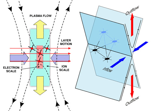
This process occurs when two magnetic fields with different or opposite orientations are directly adjacent, resulting in the disconnection of field lines and reconnection with those in the other region. This leads to a release of stored magnetic energy as kinetic or thermal energy. The reconnection process takes place in a narrow boundary between the two different fields known as the diffusion region.

MMS will focus on that particular region where the plasma becomes demagnetized and electrons decouple from ions leading to an area where electron physics dominate. However, the structure of the diffusion region is largely unknown and the processes behind the demagnetization are poorly understood as is the role of electrons in the reconnection process, the drivers behind reconnection rate, the factors that prompt the onset of reconnection, the factors that are needed to sustain reconnection and those that cause it to cease, and the fundamental processes that cause particles to be accelerated to high energies within the diffusion region in processes that can be likened to explosive transfers of energy.

Magnetic reconnection is one of the major processes in the flow of energy, mass and momentum over plasma boundaries. Therefore, an understanding of its mechanisms and drivers through in-situ measurements will provide insight into fundamental astrophysical processes.

In the Earth-Sun System, magnetic reconnection plays a major role in the generation of Coronal Mass Ejections and Magnetospheric disturbances caused as a result of CMEs leading to magnetic storms. These processes are also present in other astrophysical systems throughout the universe and reconnections is also believed to be a factor in star-accretion, disk accretion, pulsar wind acceleration and acceleration processes of cosmic rays in galactic nuclei jets. Furthermore, magnetic reconnections occurs in fusion processes as one mechanism that prevents magnetic confinement of the fusion fuel.

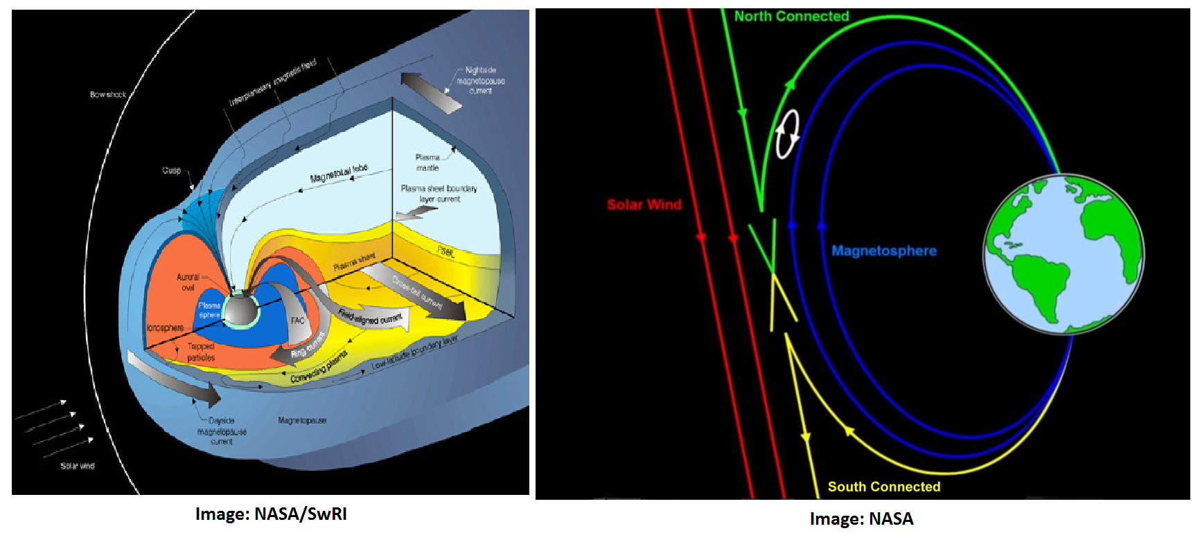
MMS uses Earth’s atmosphere as a natural laboratory to investigate the diffusion region as it occurs in a natural system since laboratory experiments produce too small of a scale size where the environments in which the critical processes operate can not be resolved. Reconnection is known to occur in the dayside magnetopause and the nightside magnetotail of Earth which will both be explored by MMS through a two-phase orbit design. Flying in formation, the spacecraft can measure the three-dimensional structure and dynamics in the heart of the reconnection region, recording particle and field parameters.

MMS is managed by the Heliophysics Division of NASA’s Science Mission Directorate while the spacecraft are built at the Goddard Spaceflight Center and the instrumentation is developed and operated by the Southwest Research Institute and its partners including the University of New Hampshire, the Applied Physics Laboratory at Johns Hopkins University, the Laboratory of Atmospheric and Space Physics at the University of Colorado, and international partners in Europe and Japan.

The MMS mission was approved in 2005 and Goddard Spaceflight Center together with SwRI were appointed to develop a detailed mission and instrument proposal.

 

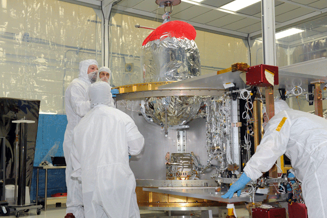
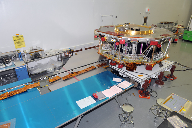
The project reached the Preliminary Design Review in May 2009 proceeding to the Critical Design Review in August 2010 that cleared the way for the construction of the spacecraft and instruments starting in 2011. In mid 2012, the System Integration Review was held confirming that the instruments were ready to start integration with the spacecraft. Integration of the four observatories with their instruments and detailed testing commenced in August 2013 on the road to a launch in the first half of 2015.

MMS Spacecraft Overview

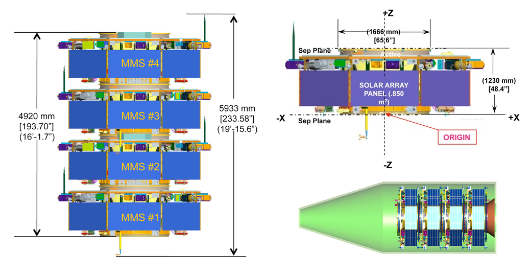
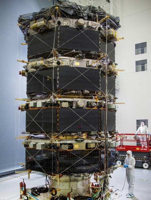
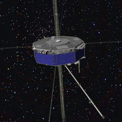
The Magnetospheric Multiscale Mission consists of four identically instrumented spacecraft, launched in a stacked fashion to enter a tetrahedral formation in an elliptic orbit around Earth set up to take the constellation through the regions of Earth’s magnetosphere that are of interest for the scientific goals of the mission, in particular the diffusion region.

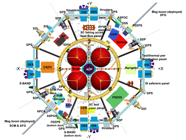
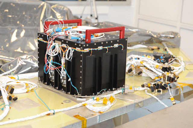
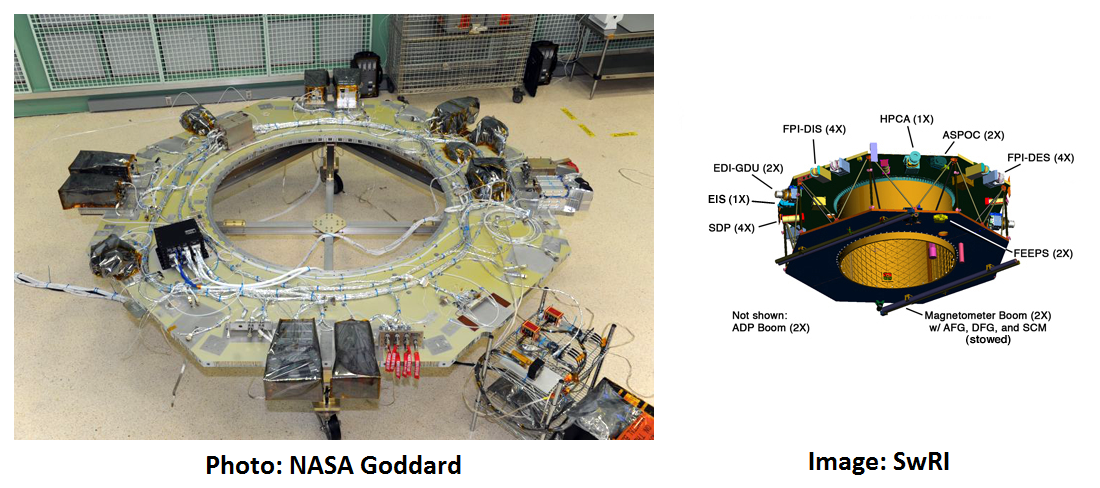
Each of the four satellites uses an octagonal platform that measures 3.5 meters in diameter and stands 1.23 meters tall with a launch mass of about 1,360 Kilograms including propellant for orbital maneuvers and formation maintenance. In operation, the satellites are spin stabilized at three RPM. Each satellite includes eight deployable booms – four 60-meter wire booms deployed in the spin plane of the spacecraft carrying electrical field sensors, two 15m axial booms also carrying electric field sensors, and two rigid booms in the spin plane facilitating the magnetometers.

The satellite platform consists of structural components made of aluminum forming the load-bearing assemblies as well as internal and external panels that can be used to mount the various satellite systems.

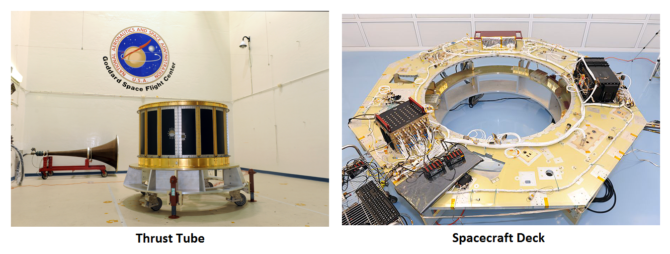
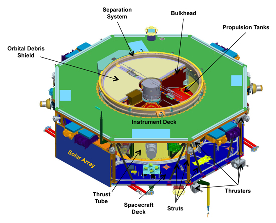
MMS uses a modular architecture to simplify the integration of the spacecraft, consisting of a propulsion system, separation assembly, thrust tube, upper instrument deck and satellite deck.

The satellite deck includes the various systems of the platform such as avionics, attitude determination and control systems, batteries, and other systems that support the instruments installed in the upper section of the spacecraft. The thrust tube in the center of the spacecraft provides the primary support during launch with all four satellites being launched stacked atop one another. The thrust tube is 1.67 meters in diameter and includes the interfaces that attach the individual satellites to each other while the lower satellite sports interfaces with the launch vehicle adapter; all interfaces include separation systems.

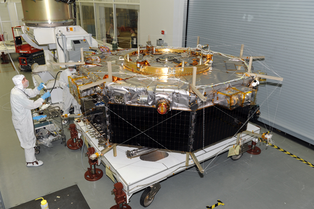
The spacecraft are equipped with eight identical solar panels installed on the side panels of the octagonal satellite platform, each panel 85 square centimeters in size.

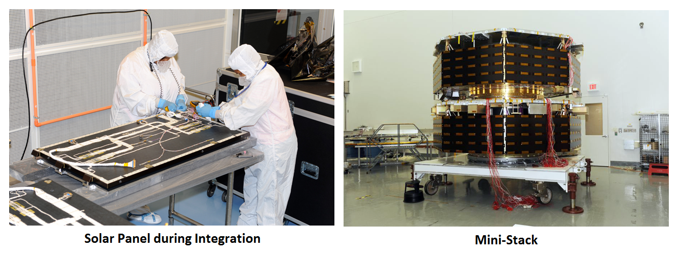
Due to the nature of the mission with fields and particle instruments, the requirements on the solar panels are relatively stringent. Therefore, MMS uses panels that are electrostatically and magnetostatically clean. The solar panels were provided by EMCORE, New Mexico, employing the company’s ZTJ technology with a conversion efficiency approaching 30%. As part of a direct power transfer system, the arrays deliver primary power to the various satellite systems during insolation with dedicated avionics conditioning the primary power bus operating at 28 Volts. A secondary Li-Ion battery delivers electrical power during the four-hour eclipse period. ABSL of Colorado built the Flight Batteries for the MMS spacecraft, each with a capacity of 68 Amp-hours and a life expectancy of over 900 charge-discharge cycles building on heritage from the Lunar Reconnaissance Orbiter and GPM spacecraft.

The Attitude Determination and Control System of the MMS consists of four Star Tracker heads, two Digital Sun Sensors, an Acceleration Measurement System AMS and a thruster system used for attitude control, orbit adjustment and formation maintenance. As a spin-stabilized spacecraft that requires precise attitude knowledge, MMS had to overcome a few challenges in the development of its ACS.

The four heads of the Star Tracker are aligned 10 degrees offset from the satellite body -Z axis with pairs of star tracker heads installed on stable optical benches on opposite sides of the spacecraft. This arrangement is a compromise between the minimization of star motion through the ST field of view and avoiding interference from the axial instrument booms deployed along the -Z axis.

An alignment transformation is applied to the output from each optical head to translate the measurements to the spacecraft body frame. Using optical sensors, the star trackers acquire four images per second that are compared with a catalog of known star constellation to determine the spacecraft attitude relative to these constellation and with that get a full three-axis orientation frame. With four ST heads, a total of 16 quarternions are provided per second, but in most spacecraft modes, attitude frames will be calculated at a cadence of one per second.

The two Digital Sun Sensors are operated in cold redundancy with one being active at a given time, delivering a pulse when the sun crosses through a narrow slit placed in the sensor field of view. This occurs once every rotation period (20 seconds) and allows the ACS controller to determine the sun elevation from the S/C body X-Y-plane.

The Acceleration Measurement System is comprised of two redundant sets of three orthogonal accelerometers that are used in the closed-loop control frame employed during delta-v maneuvers for orbit and formation maintenance, but the telemetry from the sensors can also be integrated in the attitude determination filter. The centripetal acceleration is proportional to the square of the rotation rate to deliver a measure of two components of the rate through the AMS. The AMS is installed 0.37 meters radially from the spin axis of the spacecraft.

The attitude knowledge requirement for MMS is 0.1 degrees on all axes to provide relevant pointing data for analysis of the measurements made by the various instruments measuring magnetic and electric field direction and particle flows. In reality, MMS will surpass that requirement with an expected attitude measurement accuracy of 0.05 degrees on the Z-axis and 0.02 along the X and Y-axis employing a SpinKF attitude algorithm. The attitude actuation system keeps the spacecraft within a +/-0.5-degree corridor to meet science requirements.

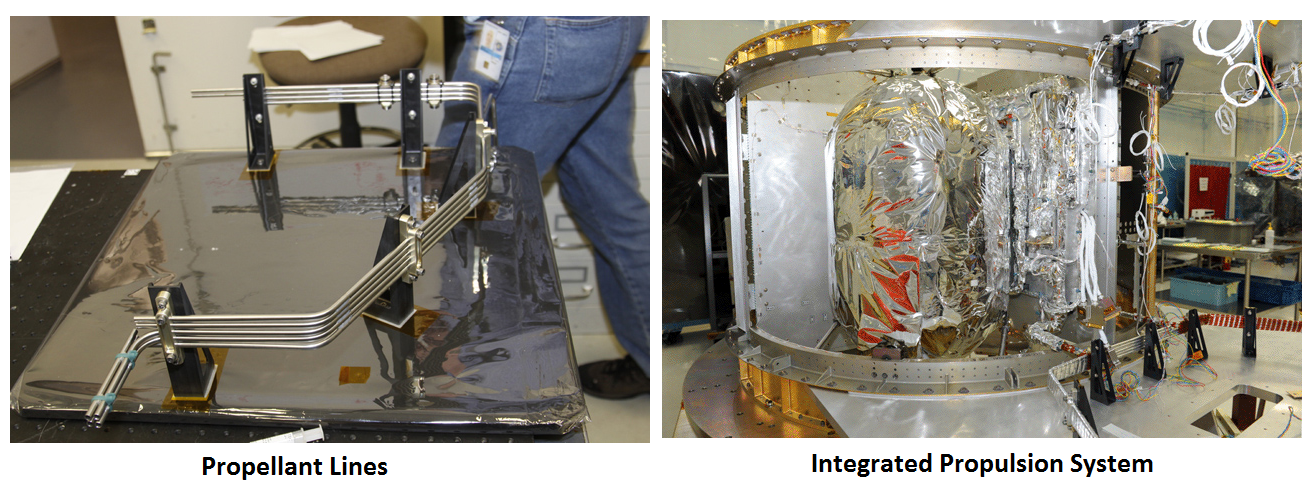
Each MMS spacecraft carries a considerable amount of maneuvering propellant to be able to complete large orbital adjustments and conduct formation maintenance maneuvers over an extended mission duration. The propulsion system consists of four titanium tanks holding Hydrazine monopropellant.

The tanks are located inside the thrust tube of the satellite and are operated in blowdown mode – pressurized prior to flight with no additional pressurization during the mission. Each spacecraft carries 360 Kilograms of Hydrazine to be consumed by 12 thrusters that use the catalytic decomposition of Hydrazine over a metallic catalyst bed to generate thrust. The thrusters are arranged in eight radial thrusters and four axial thrusters.

The radial thrusters are used for precise spin rate control, attitude control and delta-v maneuvers, providing thrust in a plane parallel to the radius of the spacecraft. The thrusters are arranged in two groups of four on opposite side panels of the spacecraft, with two thrusters of each group on the aft deck of the spacecraft and two on the instrument deck.

These eight thrusters have a nominal thrust of 18 Newtons, but operate along a range of 22 Newtons at the initial inlet pressure of 300psi down to 9 Newtons when the tank and inlet pressure is reduced to 100psi, corresponding to specific impulses of 224 seconds at the start of the mission down to 221 seconds. The thrusters are capable of operating in steady state and pulse modes.

The axial thrusters deliver a thrust component perpendicular to the plane of the spin of the spacecraft in order to be used in attitude and nutation control. Arranged in pairs on the aft and forward ends of the satellite, the axial thrusters are located in close proximity to the central thrust tube. These four thrusters are designed to deliver 4.5 Newtons of thrust at an initial inlet pressure of 325psi that is depleted to 100psi at the end of the mission with a thrust requirement of 1.5 Newtons with associated specific impulses of 227 and 218 seconds, respectively.

 

The Command and Data Handling System of the MMS spacecraft is in charge of command reception and execution, payload system operations, housekeeping operations and spacecraft control. The C&DH system uses key-components developed for the Lunar Reconnaissance Orbiter. The spacecraft uses a space wire, 1553 data bus and an analog RS-422 system for data transfer within the spacecraft. Housekeeping data and science data is stored in a solid-state recorder before downlink or is processed and downlinked in real time.

The core of the C&DH system is a Coldfire central processor operating at a clock speed of 40/20MHz and including 4MB of EEPROM holding the boot code and 12MB of local RAM to store the operating software. Housekeeping data and payload science data is stored in a 600MB Solid State Recorder.

The avionics of the MMS spacecraft are responsible for a number of operations such as command and telemetry processing, timing signal generation, power regulation, battery management, attitude determination and navigation, and thruster control. The data system uses cFE/CFS (core Flight Executive/Core Flight System) and CCSDS File Delivery Protocols.

The MMS communications system uses a dual S-Band system for redundancy. Two separate transponders are used, both capable of providing command reception and data downlink via dedicated Diplexer Units. MMS is equipped with two omni-directional S-Band antennas connected to both Diplexers via a DPDT Switch.

Total RF power is 8 Watts and MMS will be using the Tracking and Data Relay Satellites for communications during critical mission phases such as initial acquisition and boom deployments. For nominal mission operations, MMS will rely on regular ground station communication sessions to deliver stored instrument data to the ground for processing. Total data volume will be approximately 4GB per day per observatory. A single S-Band frequency is used for uplink to all spacecraft and a single frequency is used for downlink from all four satellites.

Each MMS spacecraft includes eight GPS antennas installed on each of the side panel edges to employ weak signal GPS processing for orbit and absolute position determination through GPS side lobe reception, and to deliver timing solutions to the spacecraft.

Orbit Design & Formation Maintenance

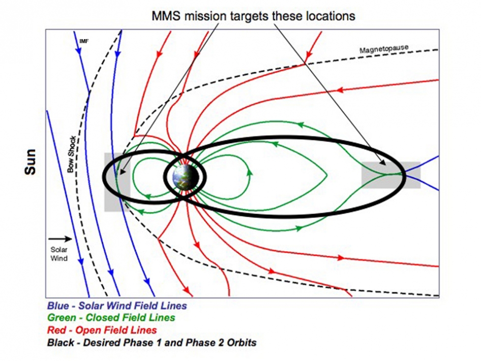
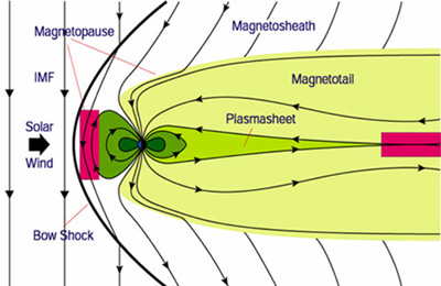
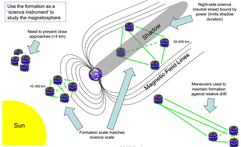
The MMS mission has been designed to maximize the time the spacecraft constellation passes through the regions of the magnetosphere where magnetic reconnection is known to occur. Reconnection manifests itself into two different locations with varying scale sizes and field orientation. In order to explore both environments, the MMS mission was developed to use a two-phase orbit strategy – the first phase focused on the mid-latitude dayside magnetopause and the second phase looking at reconnection within the nightside magnetotail.

In the mid-latitude magnetopause, MMS will be able to study the region in which the interplanetary magnetic field merges with the geomagnetic field. Here, reconnection processes account for a significant portion of the total transfer of mass, momentum and energy to the magnetopause. The solar wind inflow leads to a shift of the merged magnetic field lines of the IMF&geomagnetic field to the nightside, causing an accumulation of magnetic flux in the magnetotail – the site that is the focus of Phase 2 of the MMS mission. In this region, the spacecraft can investigate the reconnection sites where magnetic reconnection is responsible for the release of magnetic energy stored in the tail as part of explosive events referred to as magnetospheric substorms.

Reconnection in this area also allows the magnetic flux that is stripped away from the day to the nightside to be returned to the dayside through processes yet to be investigated.

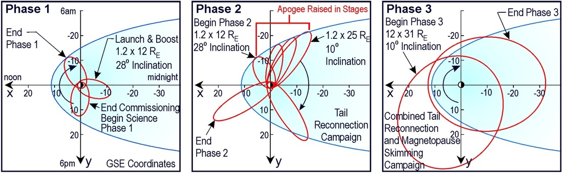
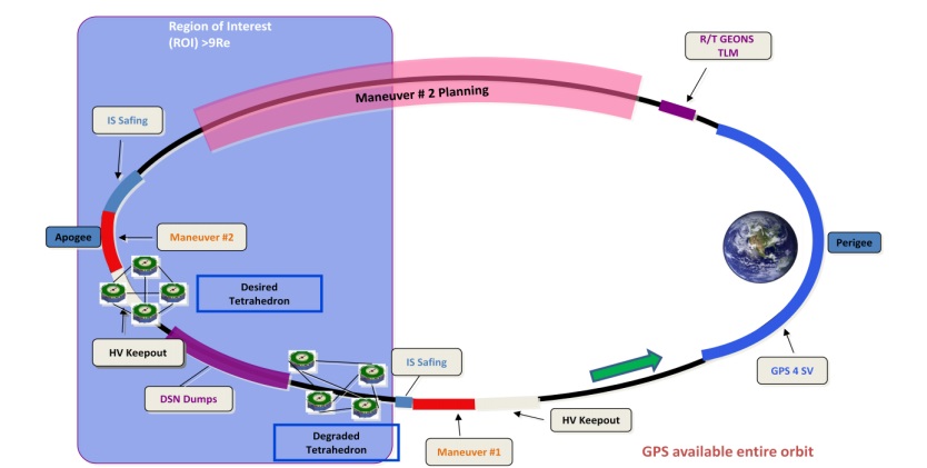
In Phase 1 of the mission, the MMS spacecraft are placed in an orbit of 2550 by 70,080-Kilometers (1.2 by 12 Earth Radii) at an inclination of 28 degrees. The formation will be flown with separation distances from 10 to 160 Kilometers and science data will be primarily recorded when the spacecraft are at an altitude of over 9 Earth Radii (57,340km) and are within 30 degrees of the Earth-Sun line on the dayside of the planet.

For Phase 2 of the mission, the spacecraft formation raises its apogee to an altitude of 25 Earth Radii, achieving an orbit of 2,550 by 152,900 Kilometers. Separation distances will be varied from from 30 to 400 Kilometers with primary science taking place when the distance to Earth is greater than 15 Earth Radii and the constellation is within 40 degrees of the Earth-Sun line on the night side of the Earth. The separation distance of the spacecraft is adjusted to match the scale sizes of the microphysical processes that occur in each region that is being studied.

In a possible extended mission, the spacecraft would adjust their orbits by raising both, apogee and perigee, and completing a plane-change to enter a 12 by 31 Earth Radii Orbit inclined 10° to study the tail reconnection and skim the magnetopause.

 

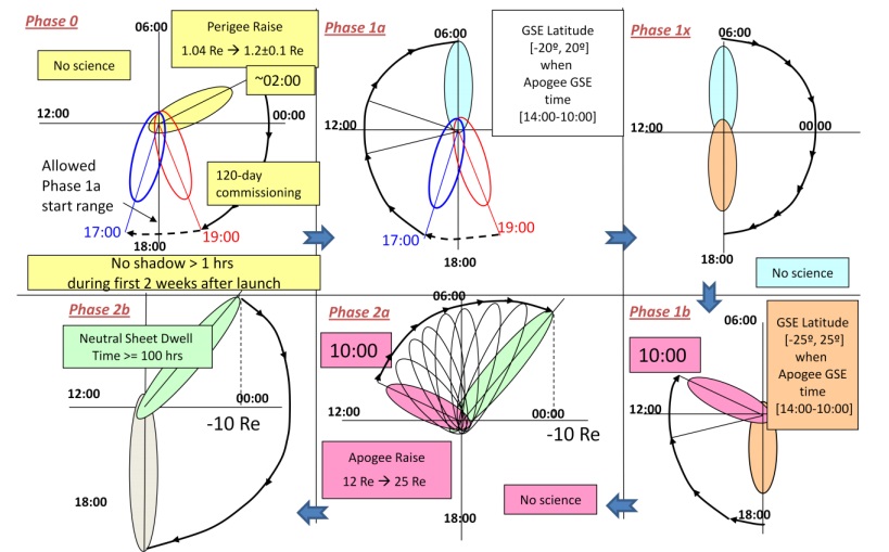
The two primary phases of the mission are connected by a transition phase during which each spacecraft completes maneuvers to raise its apogee. These maneuvers are performed incrementally by all four MMS probes to avoid separation distances to grow too large and keep the vehicles grouped together as the apogee is doubled over the course of several weeks.

The MMS spacecraft orbit the Earth in a tetrahedral formation at inter-spacecraft separation distances as low as ten and as high as 400 Kilometers, requiring constant monitoring of the progression of the orbits of each spacecraft to plan, schedule and execute maintenance maneuvers to keep the constellation flying in the expected geometry.

Given the highly elliptical orbit of the constellation, each spacecraft is subjected to natural perturbations caused by the J2 term in the geopotential mode that leads to a differential evolution of the orbit states of each probe and represents the largest natural perturbation. Another sources of gravitational perturbations can be the moon which comes into play due to the high apogee altitudes, leading to relative drift between the spacecraft and in certain geometric situations can cause a secular lowering of the perigee altitude which will require orbit adjustment maneuvers.

The natural perturbations can be calculated after the exact starting parameters of the orbital states are known and it is expected that, in theory, only occasional formation maintenance maneuvers would be needed at a cadence of one every two months. In practice, however, maneuvers will occur as frequent as once per week to once every three weeks due to errors in knowledge and execution of maneuvers that dominate over the natural perturbations.

The situation gets more complex since each spacecraft is subject to its own realization of these errors with no correlation between the four observatories. Simulation of these factors for a mission like MMS is virtually impossible which makes pre-flight prediction of maneuvers rather difficult.

To help in the precise formation flying, the MMS mission employs the Inter-Spacecraft Ranging and Alarm System, IRAS – developed at the Goddard Spaceflight Center. IRAS consists of a Navigator GPS receiver coupled with a crosslink transceiver and an UltraStable Oscillator as a frequency reference. Low strength GPS signals are acquired by the eight GPS antennas of the spacecraft to increase the number of GPS satellites that can be used from the higher altitude of the MMS orbit. The GPS-calculated position and state vector of each spacecraft is transmitted via the inter-satellite communications link and the stable frequency of the RF signal is used for ranging measurements between the individual satellites at four-minute intervals.

In charge of all calculations associated with the inter-satellite GPS and ranging data is the GPS Enhanced Onboard Navigation System Flight Software that provides orbit determination and uses GPS measurements and crosslink ranging data to determine absolute and relative orbital states. The software includes models for gravity, atmospheric drag, solar pressure, clock bias and frequency drift to provide precise estimations. The estimated state vectors are also downlinked by each satellite for planning of formation maintenance maneuvers that is completed on the ground to develop the commands needed to be sent to the spacecraft for the execution of the maneuver.

MMS Orbital Sequence

 

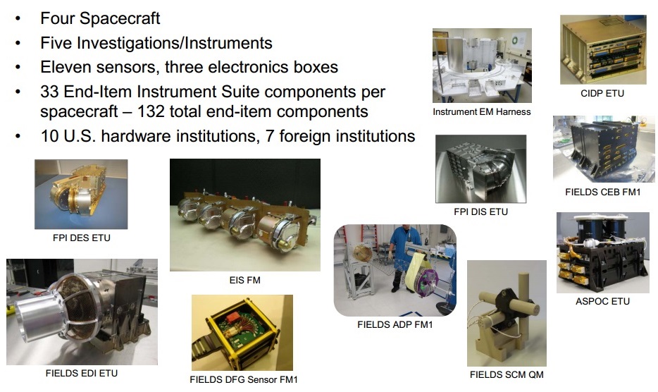
MMS Science Instruments

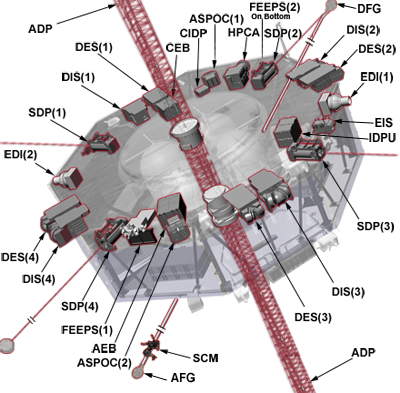
Each of the four MMS spacecraft is equipped with an identical instrument suite consisting of 11 instruments for a total of 25 sensors – installed on the instrument top deck or on the eight deployable instrument booms. The instrument suite is collectively referred to as SMART – Solving Magnetospheric Acceleration, Reconnection and Turbulence. SMART is comprised of three groups – Hot Plasma, Energetic Particle and Fields Sensors, plus two housekeeping units, the Active Spacecraft Potential Control Device and the Central Instrument Data Processor.

The MMS instrument payload measures the ion and electron distributions and electric and magnetic field properties at an unprecedented time resolution down to millisecond range as well as an unprecedented measurement accuracy at spatial scales down to 1-10 Kilometers. This will enable MMS to keep track of the fast moving diffusion regions traveling at 10-100km/s. The overall goal of the mission is to discover the mechanisms that are at work to break the frozen-in condition where the ions and electrons become demagnetized leading to the reconfiguration of the magnetic field. The mission aims to become the first to provide definitive measurements of plasma compositions at active reconnection sites while the particle detectors remotely sense regions of reconnection and determine how these processes can generate such large numbers of energetic particles.

 

 

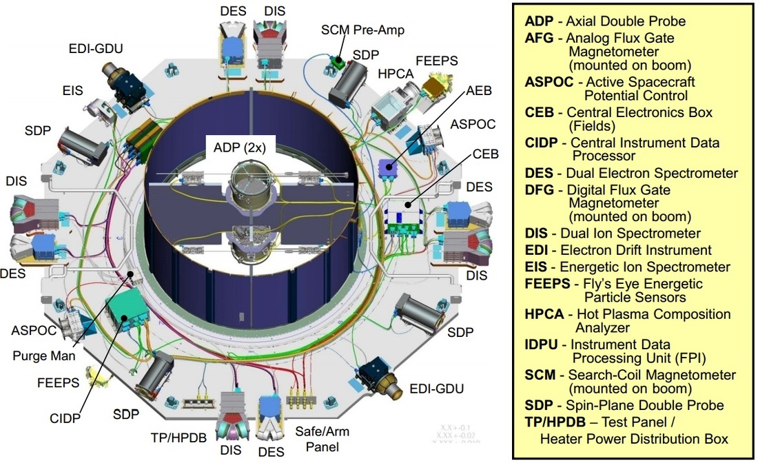
Hot Plasma Composition Suite

The Hot Plasma Composition Suite consists of four components – the Fast Plasma Instrument (FPI) comprised of Dual Ion Spectrometer (DIS) and Dual Electron Spectrometer (DES), and the Hot Plasma Composition Analyzer. Each DIS and DES Units occupies a quadrant of the MMS spacecraft, amounting to four DIS and DES units per spacecraft for a total of 32 sensors across the entire MMS constellation.

Dual Electron Spectrometer

The Dual Electron Spectrometer is capable of measuring the electron velocity distribution function for the full sky with a high-angular resolution of incoming electrons at a measurement interval of 30 milliseconds. Each DES consists of eight half-top-hat electrostatic analyzers each with a 6 x 180-degree field of view with a single pixel covering a sector of 6 x 11.25 degrees. The sensor consists of two deflectors and a Multichannel plate detector with an anode ring underneath. Two deflectors, one upper and one lower, change the path of electrons based on their energy before the electrons reach the electrostatic analyzer. The azimuth angle of impinging electrons is determined by measuring the position in which the electrons impact the Multichannel Plate detector with a position-sensitive anode while the elevation angle is measured perpendicular to the imaging plane to determine the direction of incoming electrons.

Coverage of the full sky is accomplished by stepping the field of view of each of the eight sensors through four deflection look directions.

This electrostatic aperture steering creates a +/-45 by 180-degree fan about the nominal viewing direction at 0° deflection. The two spectrometer units are installed so that their individual fields of view are set 90 degrees apart so that the FOVs created through electrostatic aperture steering cover the entire sky. The DES instruments are run in their highest time resolution mode for about 30 minutes per orbit and data processing onboard the spacecraft is done to intelligently downlink those data sets with the greatest amount of temporal structure.

DES covers an energy range of 10 electron-volt up to 30 keV with an energy resolution of 20%. The instrument provides data at a rate of 6.5 MB/s when operating in high time resolution mode.

Dual Ion Spectrometer

The Dual Ion Spectrometer is similar in design to the DES instrument, only using different voltage bias on its electrostatic analyzers.

It also covers the entire sky by employing electrostatic aperture steering and achieves the same angular resolution as DES, but it only operates at a time resolution of 150m/s, thus delivering a raw data rate of only 1.1MB/s. DIS covers an energy range of 10eV to 30 keV.

The entire FPI instrument has a data rate allocation of 1.5MB/s requiring onboard compression to be employed in addition to the intelligent selection of the most promising data.

Hot Plasma Composition Analyzer

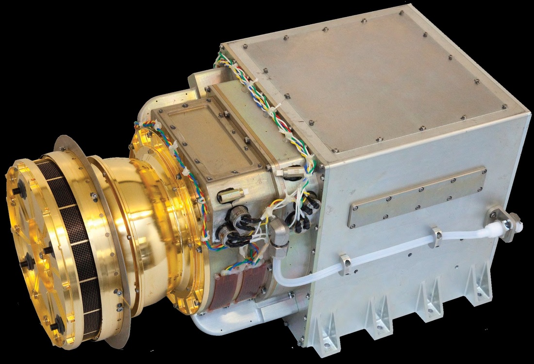
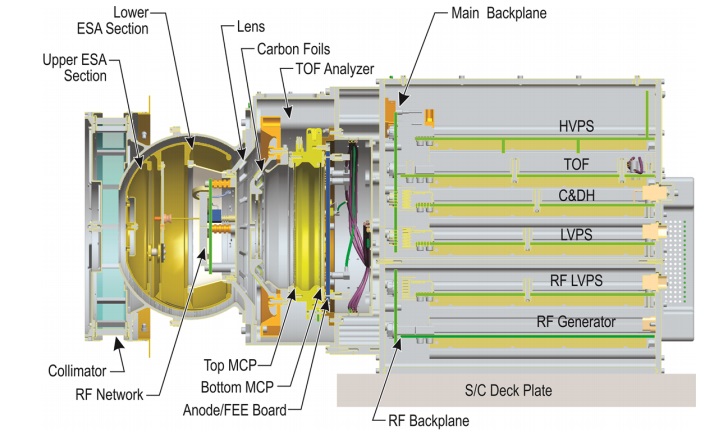
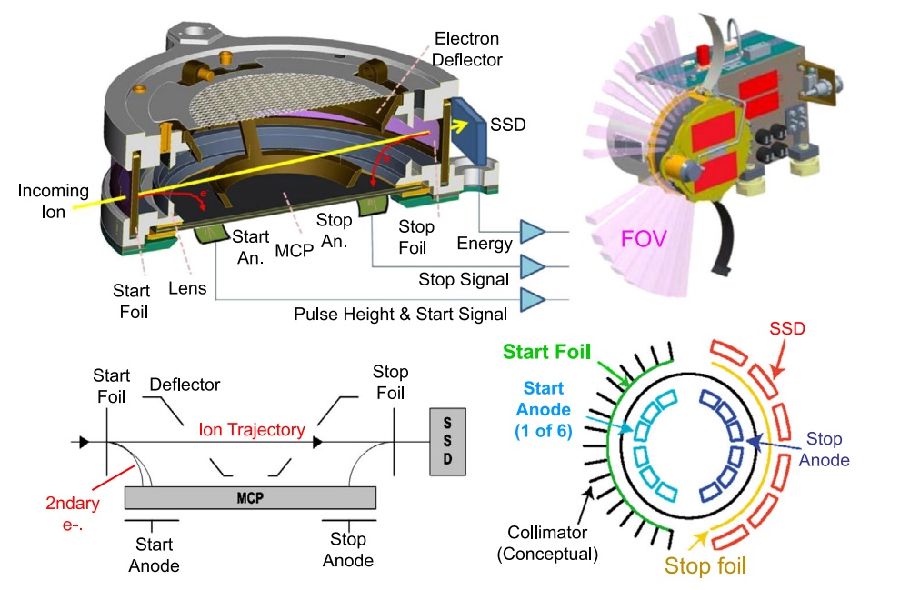
The Hot Plasma Composition Analyzer, HPCA, couples an electrostatic ion analyzer and a Time of Flight Mass Spectrometer to identify and measure the energy of ions participating in magnetic reconnection every ten seconds to deliver a three-dimensional snapshot of the highly dynamic ion diffusion region where reconnection is known to occur. HPCA is capable of separating ions that are part of the solar wind such as hydrogen (H+) and helium (He++) from those that are present in the terrestrial plasma including hydrogen (H+), Helium (He+) and oxygen (O+). Knowing the source of the plasma will allow detailed insights into plasma flow rates into the diffusion region. When outside of the diffusion region, data from HPCA can contribute to studies of geomagnetic storm dynamics.

The HPCA sensor heads consist of an aperture opening, ion deflectors, start foils and anodes, a microchannel plate detector, stop anodes and foils, solid state detectors and pre-amplifiers as well as supporting electronics.

The HPCA energy range has been chosen to be able to measure inflowing ions at low energies of 1keV to the high energy levels expected to be seen in outflow jets at up to 40keV. Measurements are done every ten seconds, or every half revolution of the observatory to obtain full-sky data.

HPCA is a toroidal electrostatic analyzer with a Time of Flight Section. It has a field of view of 90 by 360 degrees minus minor losses due to spacecraft structural obstructions. Incoming ions enter the two concentric toroids with the inner toroid having an adjustable voltage applied to match the energy of the entering ion. A particular voltage determines the energy and arrival angles of incoming ions. The entire voltage range is swept out every 615 milliseconds.

On the detector, an ion is detected on one of 16 anodes that are installed next to each other in a circular pie-type arrangement to provide ion elevation data with a sufficient resolution.

The MMS spacecraft rotation is used to sweep these 16 pixels through the three-dimensional sky to obtain a 3D measurement resolved to 256 pixels.

On each detector, a total of 32,000 bytes of data are gathered, representing a 256-pixel time-of-flight spectrum at each of the 64 energy levels.

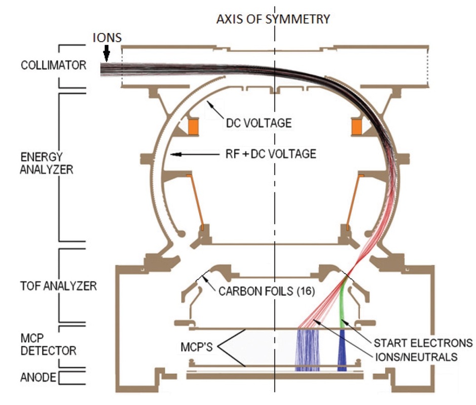
When entering the Time of Flight section of the instrument, ions are accelerated by 15keV. Secondary electrons are generated when an ion passes through an ultra-thin carbon foil at a thickness of about 50 atoms – these electrons are accelerated to a specific energy in an applied electric field and are detected in a dedicated position on the Multichannel plate detector.

When the electrons are detected, a start signal is transmitted and when the ion arrives after a travel distance of 3.4 centimeters, a stop pulse is generated to determine Time of Flight of the individual ions. This results in measured times of flight between 10 and 150 nanoseconds which, together with the energy measurement, can be used to determine the mass and with that the identity of the ion (through E=0.5m/v²). Ion flux is determined by counting the numbers of particular ions arriving per second.

One of the challenges of the HPCA instrument was the development of an effective proton rejection system due to the extremely high proton flux in the day-side magnetopause, especially in the leading edge of the magnetosphere. These energetic protons could easily damage the detectors of the instrument and have to be rejected without altering the flight path and energy of ions that are to be measured by the instrument.

HPCA employs a novel method of using a radio frequency field tuned to the frequency matching the proton velocities at their typical energy range of 1 to 4keV (400-900km/s). Traversing through the field will alter the flight path of the proton so that they hit the walls of the toroidal electrostatic analyzer. The RF does not match the velocity of the much heavier ions that are transmitted through this RF gate.

Energetic Ion Spectrometer

Two Energetic Particle Instruments are installed on each MMS spacecraft – the Fly’s Eye Energetic Particle Sensor FEEPS (two per spacecraft) and the Energetic Ion Spectrometer EIS (one per MMS spacecraft). EIS measures the energy of energetic ions from 20keV for ions and 45keV for protons up to over 0.5MeV for oxygen ions while FEEPS delivers instantaneous all-sky images of high-energy electrons from 25keV to over 0.5MeV in addition to total ion energy distribution from 45keV to 0.5MeV to provide data on all-sky ion distribution that adds to EIS data. The instruments aim to sense the position and speeds of boundaries and other structures near active reconnection sites, sense the magnetic topology of reconnection sites using electrons as tracer, remotely sense reconnection acceleration sites, and determine the cause of energization of particles by reconnection.

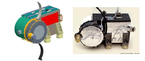
EIS carries with it a high degree of heritage from the JEDI instrument flying on the Juno Jupiter Probe. It primarily consists of a sensor head and an electronics box that are integrated as a single unit. The instrument includes electron and ion sensors and their associated detector preamplifiers. Overall, the EIS instrument weighs 2.2 Kilograms, taking up a volume of 23.3 by 16.9 by 12.8 centimeters. Its electronics box weighs 1.4kg and measures 15.9 by 20.7 by 9.3cm in size. The electron and ion sensors are arrayed in 12 by 160 degree fans with six 26.7° look directions.

EIS is installed on the payload deck of the MMS spacecraft, on the S/C interior side of the payload deck so that the instrument look direction is towards the mounting deck on the +Z axis of the spacecraft that is aligned with the +Y axis of EIS so that the instrument looks to the -Z direction aligned with -Y on EIS. A one-time deployment is performed after launch to remove a spring-loaded acoustic cover from the instrument aperture.

For the examination of ions, EIS uses an approach known as Time-of-Flight (TOF) by Energy and TOF by Multichannel Plate Pulse Height to determine the energy and velocity of ions which allow their mass to be calculated, allowing an identification of the ion species. Electrons are detected by solid state detectors that sense energy and directional distribution.

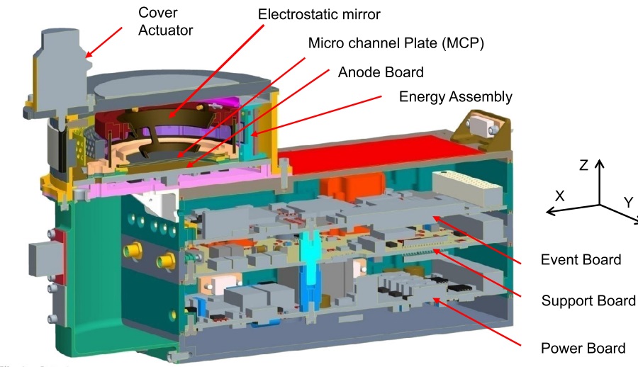
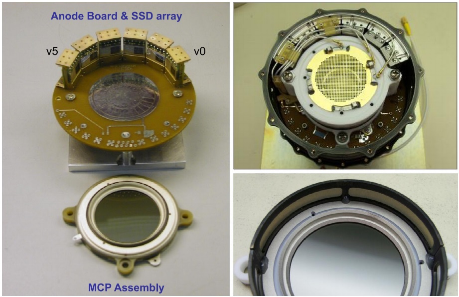
The EIS sensor heads consist of an aperture opening, electron deflectors, start foils and anodes, a microchannel plate detector, stop anodes and foils, solid state detectors and pre-amplifiers as well as supporting electronics. The EIS head includes TOF sections 6 centimeters across that feed the silicon solid-state detectors. The SSD array and the individual pre-amplifiers are connected to an Event Board that determines particle energies.

The direction of an incoming electron is determined as a function of the solid state detector that is struck by a particle, with six different viewing directions along the 160° fan; this creates an accuracy of 26.7° when measuring particle directionality which is sufficient to estimate the overall direction of particle inflow. For ions, the directionality is determined by the detection of the entrance position on the multichannel plate time-delay anode nearest to the start foil. The time delay is used in the read out across the 12 start anode pads of the instrument (connected by inductors) to measure the basic inflow direction of the ions.

As an ion enters the instrument, it first passes through a thin foil in the collimator (350A Aluminum, the collimator consists of five aluminum blades) before reaching the start foil (carbon-polyamide-carbon) and generating secondary electrons. These electrons are then directed from the primary particle path to the microchannel plate detector where the Start Signal is generated for the Time of Flight measurement. A 500-Volt potential between the foil and the MCP directs the secondary electrons to the TOF detector with high accuracy (1ns dispersion in transit time). The segmented MCP anodes with two start anodes for each of the six angular segments provide data on the direction of travel of the ion.

Secondary electrons that are created as a result of the ion passing through the stop foil (carbon-polyimide-carbon-aluminum) are again directed to the MCP and cause a Stop Signal.

The time-difference between the two signals represents the time it took the ion to pass through the 6-centimeter TOF instrument.

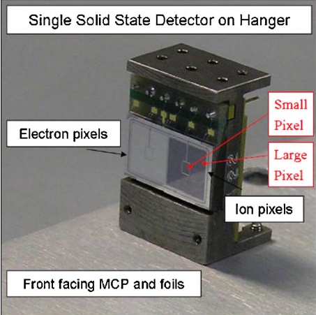
After the stop foil, ions impact the Solid State Detectors that consist of electron and ion pixels. The SSD determines ion energy which coupled with the TOF measurement delivers ion mass and particle species data. The collimator foil is installed on a high-transmittance grid (90%) supported by stainless steel frames. The start/stop foils use a tungsten-copper frame.

Electrons entering the instrument are first decelerated by a 2.6kV potential which is part of the TOF system for ion measurements. After passing the stop foil, the electrons are again accelerated by a 2.6kV potential. Reaching the SSD detectors, the electrons are detected in the electron pixels that can measure electrons at energies of 25 keV to 1 MeV. The electron detectors are covered with 2-micrometer aluminum metal flashing to reject protons at low energies under 250keV. Electron measurements do not require a TOF measurement because direction is directly measured by the detector.

The Microchannel plate stack inside the EIS instrument includes two 5-centimeter diameter plates mounted with a small 0.25cm gap in between. The stack is operated at potential drops between 1900 and 2400 volts with a segmented anode collecting the flow of electrons out of the stack. The individual MCPs are connected with time-delay inductors.

The detector system has to be time-multiplexed and can either measure electrons or ions. Three species modes (electron energy, ion energy & ion species, all coupled with direction measurements) are cycled on a commanded interval of 0.67 seconds (1/32 of a spacecraft spin) or based on programmed event triggers. The six physical SSDs provide a total of 24 SSD pixels (every SSD has 2 electron and two ion pixels – one large pixel of 6.2 by 6.5mm and a small pixel in the center of 1.3 by 1.6mm). The small pixels represent a relic of the JEDI instrument for Jupiter, and will likely not be utilized in the primary MMS target regions. The SSD is about 500 microns thick with a 500-Angstrom dead layer. The entire SSD array is about 3.4 centimeters in diameter. Each SSD is connected to a Preamp Board that is part of the sensor assembly.

The electronics box of the instrument holds the event board, power supplies and support electronics – the boards are printed circuit boards measuring 10 by 15 centimeters. The Event Board interfaces with the sensor to receive TOF signals, SSD data, and MCP pulse heights that are processed by a RTAX2000 16-bit, 10MIPS processor with 512KB SRAM and interfacing with a 64KB PROM and 256KB EEPROM.

It puts the signals coming directly from the detectors through analog to digital conversion and employs science data processing filters, reading events out to a Field Programmable Gate Array that uses an event-logic to determine look direction, particle energy and particle velocity. A dedicated Low Voltage Power Supply delivers the low-voltage buses for the various electronics of the sensor while the high-voltage is provided to the sensor head via a High Voltage Supply and Monitor Unit. The Support Board hosts the command and telemetry interface with the MMS spacecraft and it also includes the PROM and EEPROM holding the FPGA boot code. Data and commands between the instrument and the spacecraft are exchanged via an RS-422 link. Overall, EIS can process 30,000 events per second.

Fly’s Eye Energetic Particle Detector

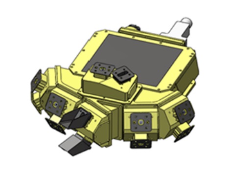
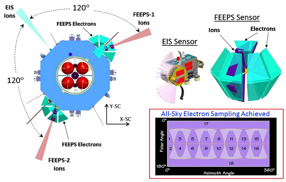
The Fly’s Eye Energetic Particle Sensor FEEPS includes a total of nine viewing sectors pointing to different directions to make instantaneous all-sky measurements of the electron and ion energy distribution in the different arrival directions. FEEPS uses silicon solid state detectors that absorb the energy of incoming particles which create a current that can be measured to determine the energy of the particle. With two FEEPS instruments mounted on two opposite sides of the instrument deck of the MMS spacecraft, the instrument can achieve a nearly complete view of the sky.

The electron sensors of FEEPS are placed so that a complete coverage in all directions is achieved with a high angular resolution that is achieved by taking a total of 64 samples per spacecraft spin for all of the electron sensors. With two FEEPS and one EIS Instrument, the spacecraft has a total of three ion viewing sectors (fans) spaced 120 degrees so that when the spacecraft is spinning, a complete sky coverage is achieved every seven seconds.

The FEEPS electron sensors are comprised of an entrance slot followed by a 1.8-micron aluminum foil for proton rejection at energies lower than 250keV. The foil allows electrons at energies of over 25keV to pass while rejecting protons at these lower energies. The transmission of protons over 250keV can lead to data contamination in certain conditions such as transient solar proton events. Behind the foil resides the 1-millimeter thick solid state detector that detects the energies of the arriving electrons.

The ion sensors also consist of entrance slots that are followed by 8-10-micron solid state detectors. The SSDs are manufactured as thin as possible to minimize their response to electrons since high-energy electrons penetrate the SSDs and leave behind energies below the detection threshold.

FEEPS measures electrons at energies from 25keV to 500keV and ions from 45keV to 500keV at a time resolution of under ten seconds. The instrument will deliver the total electron flux density and the heavy ion integral directional flux.

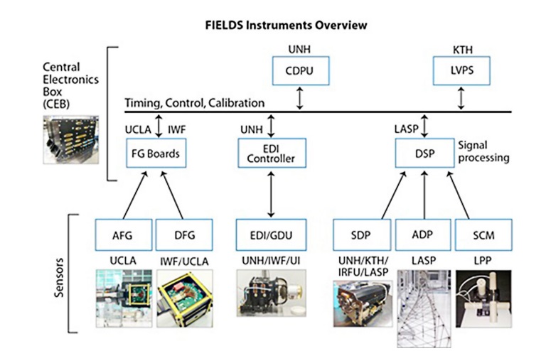
FIELDS

The Fields Investigation is a suite of six sensors to provide the critical measurements of the electric and magnetic field direction and intensity around the individual MMS spacecraft. FIELDS includes a Central Electronics Box that supports all sensors that are part of the instrument suite. Inside the box is a Low-voltage Power Supply that delivers power to the various instrument electronics of the instrument suite, a Central Data Processing Unit that receives data from all sensors and transmits it to the spacecraft mass memory for downlink. Also inside the CEB are the individual controllers of the instruments that command the sensors and receive data from them.

Digital Fluxgate Magnetometer & Analog Fluxgate Magnetometer

 

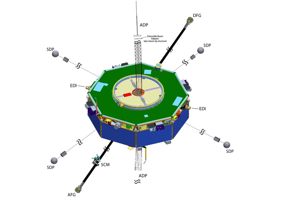
Each MMS spacecraft features two independently designed fluxgate magnetometers to avoid single point failures given the high priority of obtaining measurements of the magnetic field vector and field intensities which is critical for the success of the MMS mission. The two magnetometers are the Digital Fluxgate Magnetometer DFG provided by the Austrian Academy of Science and an Analog Fluxgate Magnetometer AFG from the University of California. It was important to include very different magnetometers that use different heritage and operating principles to ensure continuous and valid data could be acquired.

All objectives of the MMS mission require a precise measurement of the magnetic geometry and magnetic currents present on a small scale and a larger scale measured across all four spacecraft. Although two different magnetometers are part of the mission, the instruments are operated by a single team and all data is shared and constantly inter-compared.

The two triaxial fluxgate magnetometers are installed on two 5-meter booms that are deployed into the spin plane of the MMS satellite. The booms are mounted on opposite sides of the spacecraft. It is important to move the magnetometers as far away from the spacecraft body as possible since the various electronic parts on the satellite create their own magnetic field that can contaminate the measurements made by the precise magnetometers, even if being factored into data processing.

The overall principle of the two fluxgate sensors is identical – making use of the nonlinearity of magnetization properties for the high permeability of easily saturated ferromagnetic alloys to serve as an indicator for the local field strength. The ferromagnetic material is surrounded by two coils of wire – one coil runs an alternating electrical current which drives the core through an alternating cycle of magnetic saturation. This changing field induces a current in the second coil which can be measured by a detector.

In a magnetically neutral environment, the input and output currents would be identical, but the presence of an external field leads to an easier saturation of the core when in alignment with the core while saturation is less easily achieved when the core is exposed to an opposing field.

This leads to the output current becoming out of step from the input which, with the known parameters of the core material and the simultaneous measurement of the input, will provide information on the local field strength using known calibration data.

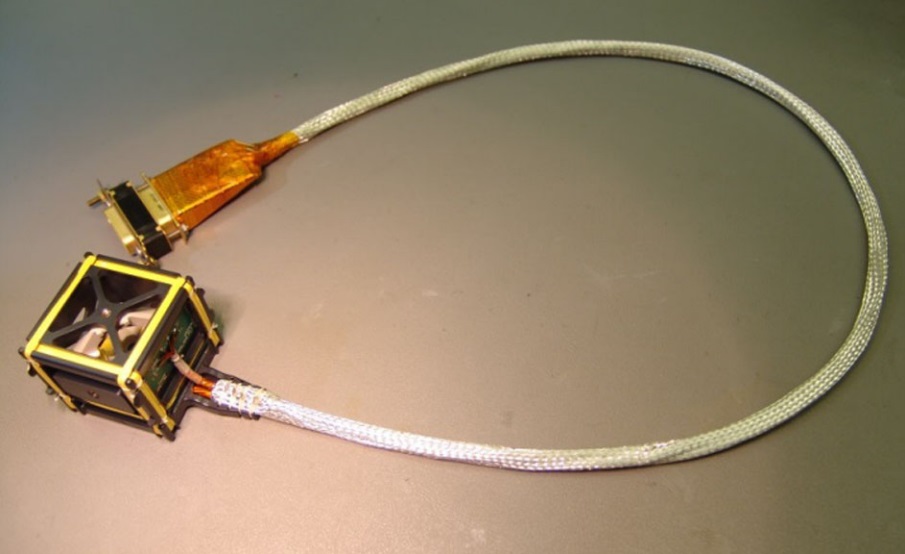
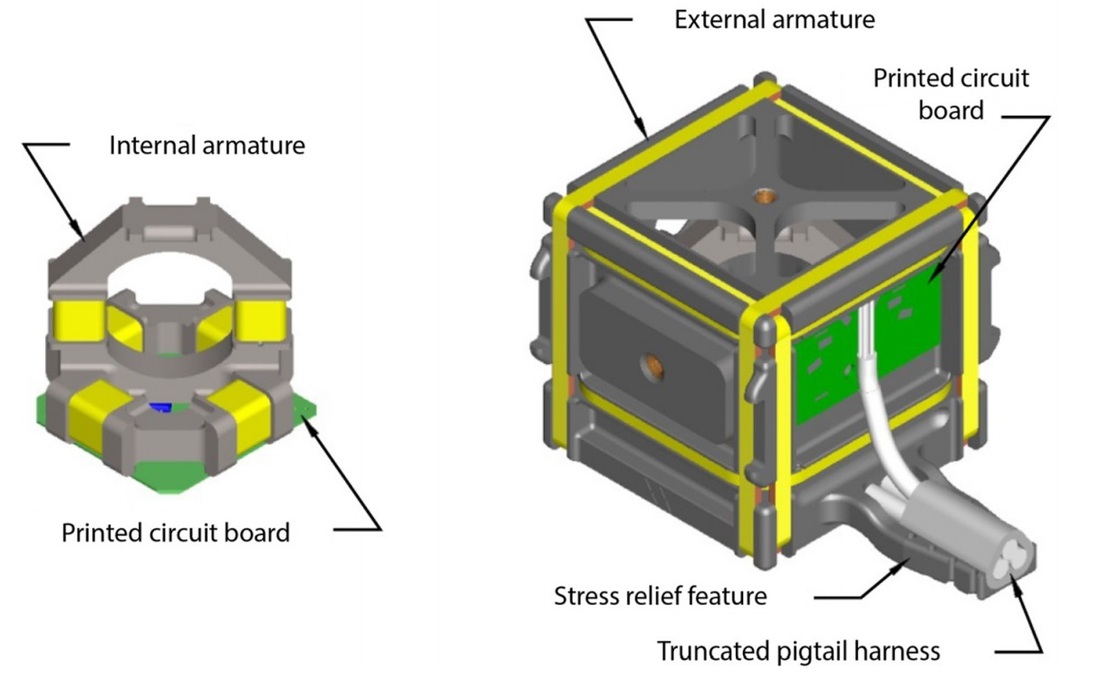
Using this basic working mode, the two magnetometers consist of two magnetic ring cores, processing wire windings that drive the cores into saturation and another set of six wire windings to sense the time-varying magnetic flux in the cores, plus a set of ambient field canceling wire windings that allow the instrument to operate in a feedback mode. Each sensor weighs 64 grams and is 4.24 by 4.43 by 4.87 centimeters in size while the truncated pig tail harness has a mass of 88 grams and is 72.5 centimeters in length.

In its feedback mode operation, the sensor cyclically measures the sense winding signal (that scales with the present ambient magnetic field) and drives current into the feedback coils in order to cancel that field out, again detecting the winding signal and searching for a minimum. The output signal of the field strength required by the feedback coil to cancel the ambient field.

The sensors of AFG and DFG are identical and based on a robust and well-known design while the electronics units of the two instruments are of different heritage. This avoids a common fault in one type of instrument taking out the entire magnetic field measurement which is an absolute essential requirement for MMS to meet is objectives.

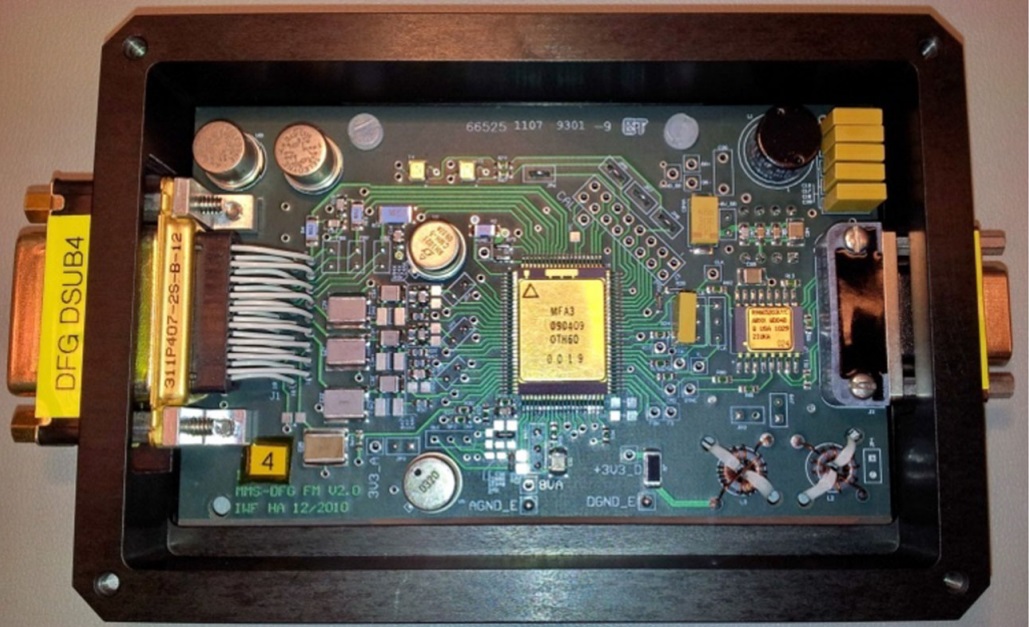
The Digital Fluxgate Magnetometer DFG is built around a miniaturized Application Specific Integrated Circuit that is the central part of the Magnetometer Front ASIC MFA. The MFA houses all active electronics that are needed for the readout of the sensors and the digitization of the sensor output. Other components of the DFG are driver components for the digital interface and the excitation of the fluxgate sensor, a voltage reference and a voltage regulator. The entire DFG electronics board measures 11 by 7 centimeters and interfaces with the AFG sensor electronics that is inside the Fields Central Electronics Box.

The analog portion of the MFA includes 14,000 transistors and contains four sigma-delta modulators for a high-resolution analog to digital conversion. Three modulators interface with the fluxgate sensor to tune the MFA to the sensor while the fourth is connected to the output of an eight-to-one multiplexer that delivers outputs from housekeeping sensors such as thermistors. The modulators deliver a single-bit output that is processed by a digital tuning logic outputting noise-shaped and digitized signals with 6-bit data width at a sampling rate of 8,192 Hz.

The digital portion of MFA hosts 25,000 gates and includes 128MHz primary and secondary decimation filters up to 64MHz output. The MFA can handle a radiation dose over 300krad and remain functional.

The DFG instrument operates in two dynamic range regimes of +/-650nT and +/-10,500nT. The lower dynamic range will be in use most of the time as it provides data at a higher sensitivity and lower noise.

The Analog Fluxgate Magnetometer AFG consists of three primary elements, the precision low mass sensor, the interconnecting boom cable and the electronics board. In addition to the analog-to-digital processing of the AFG sensor output, the electronics board of AFG also delivers power, timing signals, commands, and data to the DFG electronics from the FIELDS package that delivers power and timing for all Fields instruments and receives data from the individual instrument payloads that are part of this particular package.

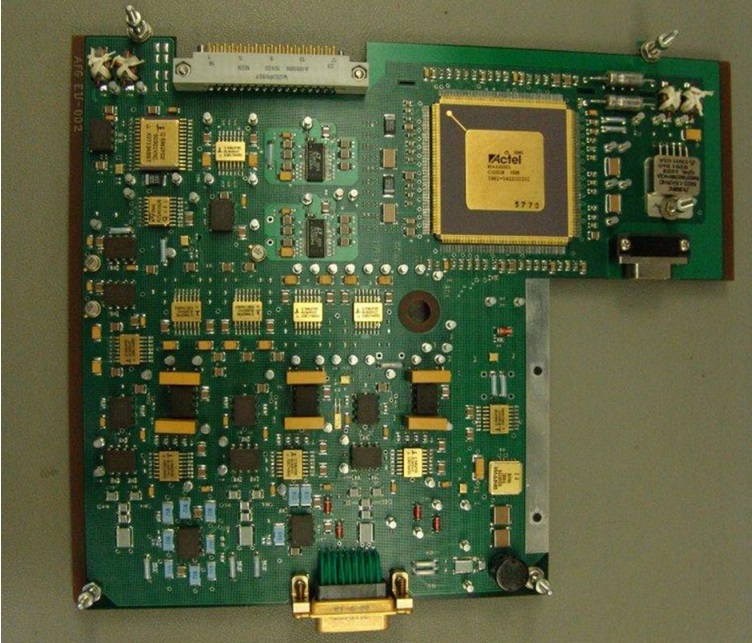
The electronics board of the AFG instrument is 23 by 19 centimeters in size and weighs 285 grams. AFG is comprised of the fluxgate analog circuit, analog to digital converters, digital circuitry, spacecraft interface circuit, and power monitoring and conditioning units. The circuit produces a drive frequency of 16kHz and detects the 32kHz second harmonic that is created by the sensor when an ambient field is present. This signal is multiplexed and sampled by a LRC1604 16-bit analog to digital converter.

AFG samples each axis 16 times in 60 microseconds which is put through a filter to generate a 24-bit sample at a rate of 128Hz. The three sensors for each axis are sampled sequentially and a 16x amplifier can be used to provide high-resolution low range data. The A-D processing is completed by an RTAX2000 Field Programmable Gate Array and two LT1604 converters. The data provided by AFG consists of the magnetic field values for the three axes, status telemetry and the housekeeping vector.

Depending on the ambient field, AFG can be commanded between full scale ranges of either +/-510 nanotesla or +/-8,200nT. Most science data will be gathered in the low range that has a lower noise and increased sensitivity. The instrument provides an excellent stability with a drift of under 0.1nT over 100 hours.

Electron Drift Monitor

The Electron Drift Instrument EDI determines the electric and magnetic fields in a different way than all other sensors installed on MMS using a geometric measurement method for the electric field and a timing method for the magnetic field. Two EDI units are installed on opposite sides of the payload deck of each MMS spacecraft.

Two Gun Detector Units in each EDI unit emit an electron beam that drifts into the direction of the combined electric and magnetic field (E x B) and, if directed properly, returns to the spacecraft after one or more gyro-periods. Is the drift-step, defined by the drift velocity and gyroperiod, on the order of the baseline separation of the two Gun Detector Units, then the electric field can be determined by a triangulation method.

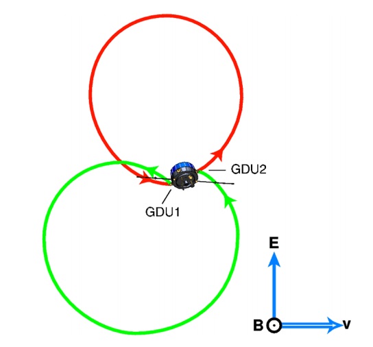
The first Gun Detector Unit emits a beam that is detected by the other unit and vice versa. The drift is the displacement of the intersection of the two electron beams from the position of the detector. To identify the emitted electrons from any ambient electron sources, the beams are pseudo-noise encoded.

In the Time of Flight Mode, the difference in the time of flight of the two beams is determined which provides the magnitude of the drift step with the gyroperiod calculated from the average of the two times. The magnitude of the magnetic field can be computed from the gyroperiod while the directions of the successful beams are used in the calculation of the direction of the magnetic field vector.

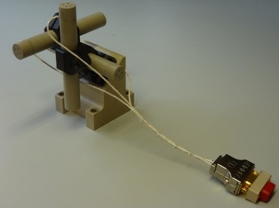
EDI consists of three main parts, an instrument controller, and the two Gun Detector Units which are comprised of the electron gun, electron optics, a sensor and a correlator. In order to measure the electric field, the fluxgate magnetometers of the MMS spacecraft supply EDI with the currently measured magnetic field direction so that EDI can use this information to determine the plane perpendicular to the magnetic field. The electron gun sweeps across this plane until the pseudo-noise encoded beam returns after one gyration.

The electron guns generate a weak electron beam with an angular width of 2° and an energy of 1keV. The beam can be steered in any direction over a hemisphere. Modulation of the electron beam occurs between 50kHz and 4MHz. The deflection of the electron beam is accomplished through the use of electrostatic deflectors that have their voltages adjusted based on the calculation of the target plane for the electron beam that is determined from the measured magnetic field direction.

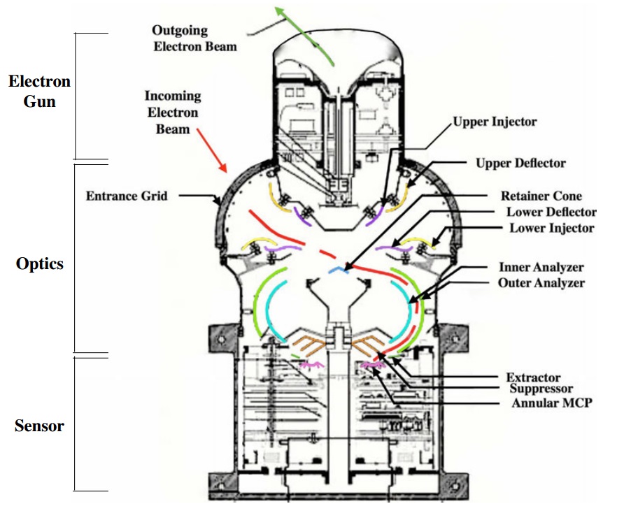
The incoming electron beam enters the instrument optics through a high-transmission copper beryllium entrance grid that forms a grounded basket used to shield the plasma surrounding the spacecraft from the voltages inside the optics of the electron sensors. Five voltage surfaces are part of the detector, injectors, deflectors, retainer cone and analyzers that are constantly having their voltage adjusted based on the emission direction of the electron beam and the local magnetic and electric fields. This is done so that the five voltages of the entrance optics deliver the incoming beam to the same position in the opening of the analyzer optics which allows the four voltages inside the analyzer to remain unchanged for most of the time.

Entering the deflector, an upper and lower deflector bend the beam to the center of the detector on a path that is further refined by the upper and lower injectors that place the electrons on a path towards the retainer cone which sets the position of the incoming electrons in the y-direction so that the electrons use a shared entry point into the analyzer. The electrons then pass downward into the annular Microchannel Plate Detector for amplification and counting. A suppressor and extractor are used to attract the electrons toward the MCP by a voltage drop an the suppressor prevents backscatter to ensure all electrons strike the detector.

The sensor, located below the MCP, consists of 32 anode pads creating a resolution of 11.25° for the measurement of the direction of the incoming beam that is measured as a function of the pad that is hit. The number of particles hitting the detector is determined through the MCP that amplifies each electron so that the sensors can read the current pulse created by the electrons that is then digitized for read-out.

The pulse signal is processed in the correlator that compares the beam’s initial modulation to what is received by the detector to determine whether the pattern matches and the time of flight equals one gyroperiod.

The advantage of the EDI sensor is that the electric and magnetic fields emitted from the spacecraft do not have a large effect on data contamination since the gyroradius is on the order of several Kilometers where spacecraft fields are non existent. EDI makes about ten measurements per second.

In addition to detecting the electrons emitted by the instrument itself, EDI can also detect ambient electrons at 1024 samples per second at energies of 0.5 to 1keV.

Search Coil Magnetometer

The Search Coil Magnetometer SCM measures the three components of the magnetic fluctuations from 1Hz to 6kHz which includes kinetic Alfvén waves, whistler mode waves and solitary waves. Data from SCM will be used to determine the contribution of plasma waves to the turbulent dissipation that occurs in the diffusion region. SCM resides four meters out on the AFG magnetometer boom.

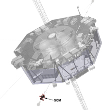
The SCM consists of a three-axial set of magnetic sensors, associated pre-amplifiers residing in a box installed on the spacecraft deck, a Digital Signal Processor and Low-Voltage Power Supply, both installed in the Central Electronics Box and shared with other FIELDS instruments. SCM operates on an eight-volt power supply.

The SCM instrument consists of three sensors that are mounted in a triaxial configuration to be able to measure magnetic field properties along all three axes. The sensors are precisely aligned with respect to the satellite axis and the orthogonality between the three sensors is better than 0.05 degrees. After problems were found in the alignment of the sensor with the spacecraft axis that were introduced when installing the instrument on the AFG boom, precise measurements of the alignment errors were taken to be factored into data processing.

Each magnetic search coil consists of a fine copper wire wrapped over ten thousand times around a 10-centimeter long, 4-millimeter diameter ferrite-metal ferromagnetic core. The primary copper winding collects the voltage induced by the time variation in the ambient magnetic flux. A secondary coil with a lower number of windings is used to provide flux feedback, removing of the resonance and flattening the frequency response of the antenna. The feedback control also removes the phase variations associated with temperature variations.

Around each antenna, electrostatic shielding is used, reinforced by multilayer insulation that ensures a thermal isolation of the sensors. The total mass of the SCM sensor is 214 grams.

The three analog voltage signals from each sensor are routed to the preamplifier box on the payload deck of the spacecraft. The cable harness is outfitted with a silver-plated copper conductive shield braid. Each voltage channel goes through two stages of preamplification – the first stage uses a low-noise input at a gain of 46dB, the second has a gain of 31.5dB for low and high pass filtering. An onboard calibration signal is supplied from the Digital Signal Processor.

Double Probe Instruments

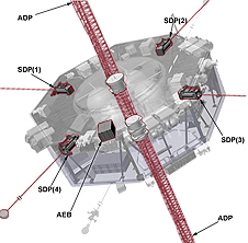
The MMS mission requires two sets of double probe instruments – the Spin Plane Double Probe installed on four 60-meter booms with spherical sensors at their ends, and the Axial Double Probe installed on two 15-meter antenna booms that are deployed axially along the spacecraft spin axis. The overall goal of the combined SDP/ADP instrument is the measurement of the three-dimensional electric field with an accuracy of 0.5mV/m over a large frequency range up to 100kHz.

Measuring the electric field is of great importance since it is responsible for the acceleration of charged plasma and therefore plays a significant role in the dynamics of magnetic reconnection, the process of converting electromagnetic energy into intense bursts of kinetic energy. The measurement of the electric field parallel of the reconnecting layers can provide a direct determination of the reconnection rate. The measurement of the electric field spectrum of plasma waves is also important to understand wave modes that cause scattering of plasma particles that creates an anomalous resistivity mimicking the resistive properties of conductive plasmas.

Spin-Plane Double Probe

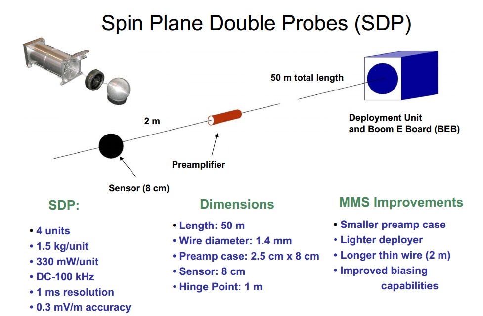
The Spin Plane Double Probe SDP measures the electric field in the spin plane by sensing the potential difference between the four current-biased spherical titanium-nitride ball electrodes installed at the end of the 60-meter long boom assemblies mounted at a spacing of 90°.

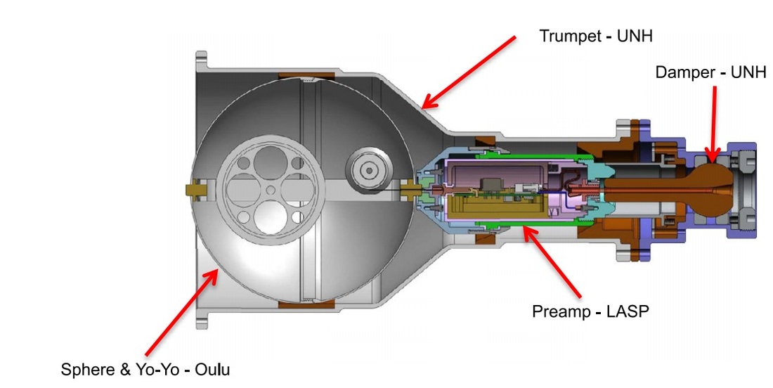
The thin 1.55-millimeter wire booms have a length of 57 meters and interface with the boom deployment assembly mounted on the spacecraft deck and the upper segment of the boom that is deployed outboard. This upper segment includes a preamplifier that is connected to the 8-centimeter ball electrode via a 1.75-meter titanium wire. This creates a total distance between two opposite ball electrodes of 120.92 meters, although the effective base length will be smaller due to the influence of the boom system on the measurement which will be factored into ground processing algorithms. One SDP unit weighs 4.3 Kilograms.

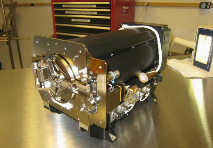
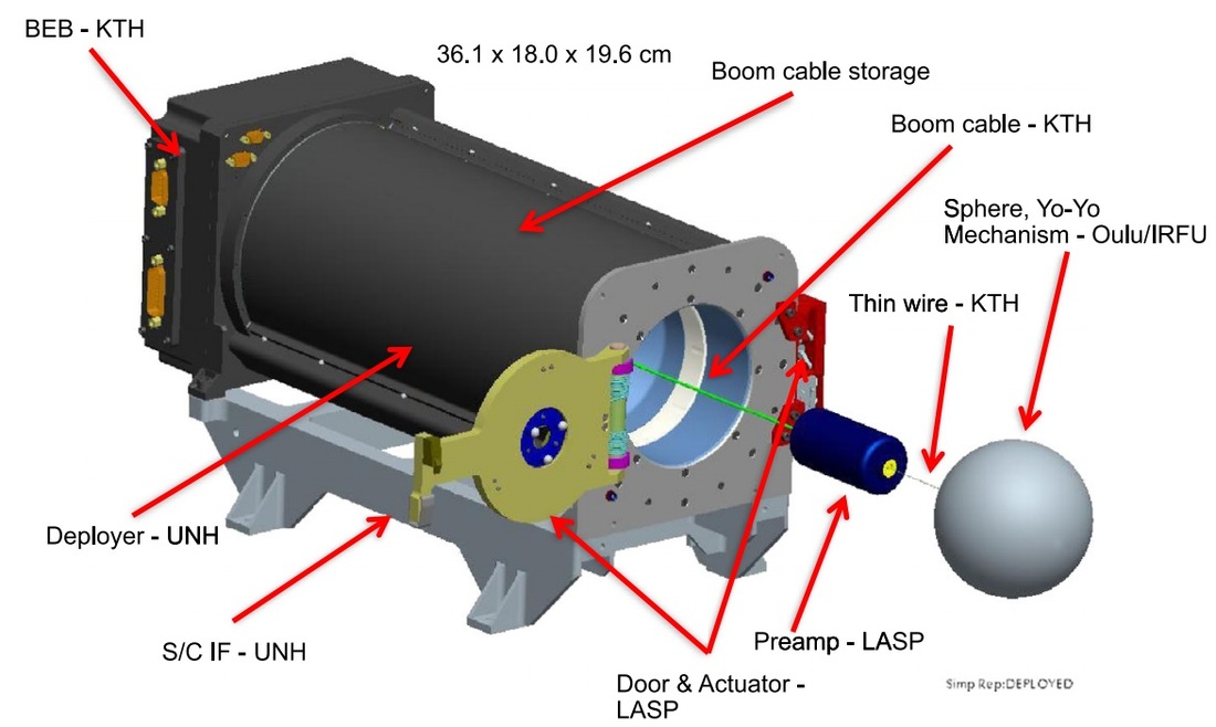
At the base of each boom is the deployer that houses the entire boom assembly including ball electrode and preamp when in the stowed configuration; it also includes the boom electronics boards. The boom cable is stowed between two concentric cylinders inside the deployer with a deployable door enclosing the assembly. Overall, the deployer measures 36.1 by 18.0 by 19.6 centimeters.

For the deployment, the boom cable is fed through the back end of the deployer by a stepper motor. Strain gauges are used to monitor the torque in the gearbox during the deployment and an inductive sensor on the main deployment wheel measures the deployed length. A damper serves as the hinge point of the boom in its fully deployed configuration to dampen loads from the spacecraft to the boom, particularly during propulsive maneuvers.

The Ball Electrode is held inside a trumpet in the inner cylinder of the deployer, inside the ball probe is a Yo-Yo that holds the 1.75-meter thin wire to be deployed as part of the initial release sequence once the probe exits the deployer.

For the deployment, the four doors on each deployer are opened, the four boom cables are deployed to 17 meters with several steps followed by the spin-up of the spacecraft to 7RPM to deploy the 1.75m thin wire and continuing the deployment of the boom cables to 41 meters on opposite boom pairs in a series of steps. Afterwards, the spin rate is adjusted to 6.1 RPM and the final deployment of the boom wires to 57 meters is completed ahead of the spin-down of the spacecraft to 3 RPM.

The boom cable itself is comprised of 7 individual electrical connectors that are bundled inside a conductive braid – the conductors have a polyimide insulation and six Kevlar strands are routed around the conducting wires to carry the pulling force of up to 200 Newtons per strand. An aluminum-kapton foil and silver-plated braided shield surround the inner strands of the boom wire.

The preamplifier has to be installed close to the sensors to avoid losses, it is cylindrical in shape with a diameter of 3.1 centimeters and a length of 7.1 centimeters. It provides a low impedance unity-gain signal of the sphere’s potential to the instrument electronics that are on the base of the long boom. The preamplifier casing is made from coated aluminum and is divided in an inner&outer guard that is biased between -10 and +10 Volts with respect to the sphere in order to influence the flow of photoelectrons to and from the sphere to optimize the electric field measurements. The unity gain signal is used to drive the outer conductors running around the primary signal wire to reduce the effective capacitance of the long wires running the entire length of the boom up to a frequency of 300 Hz and voltages from -80 to +100V.

The thin titanium wire leading from the preamp to the sphere is 0.24 millimeters in diameter and consists of 19 individual strands. It is galvanically connected to the sphere and thus has the sample electrical potential. The 8cm probe is made from titanium and nitrided at 800°C to create an titanium nitride surface. The spherical shape and uniform surface of the probe is required for a good electric field measurement as the spacecraft spins the individual part of the surface in and out of sunlight.

Inside each probe is a Yo-Yo mechanism that holds the thin titanium wire when in its launch configuration. All surfaces of the Yo-Yo are gold-coated to ensure good electrical conductivity and a spring-loaded main reel deploys the wire – carefully tuned to match the required force on the thin wire before, during and after the deployment.

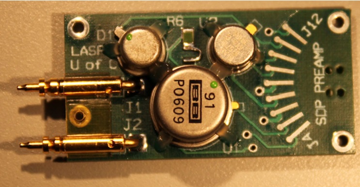
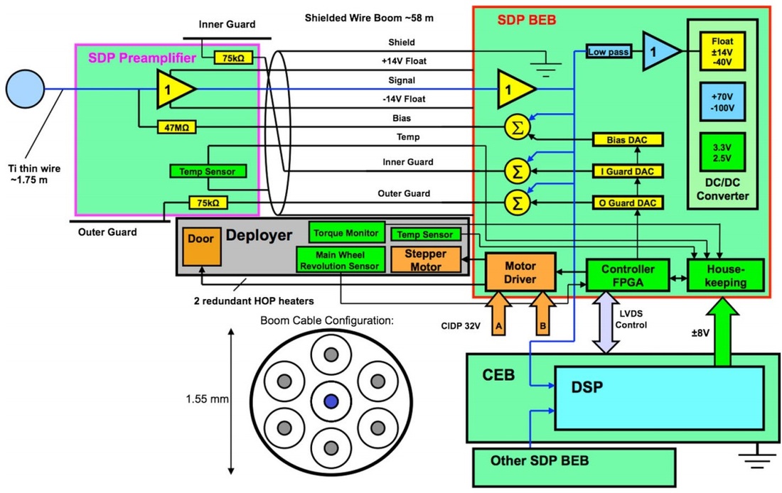
The SDP electronics are facilitated on four electronics boards – 3 Boom Electronics Boards housed in the deployer on the spacecraft deck and 1 Preamp Board inside the Preamplifier out on the boom. The electronics are in charge of controlling the bias current that keeps the probe near the ambient plasma potential, controlling the preamp outer and inner guard surfaces, to amplify the probe signal, to transmit the analog signal to the Digital Signal Processor, receive and execute commands from the Central Data Processing Unit, sending housekeeping data to the FIELDS CDPU, controlling the stepper motor for boom deployment, monitoring the torque and deployed length, measure the boom cable deployed length by the number of turns of the deployment wheel, and relay power to the instrument components.

The Boom Electronics Boards are comprised of a Control and Power Board that receives power from the Central Electronics Box power supply and converts it to the voltages needed by the SDP using DC/DC converters operating at a frequency of 211kHz. An Analog and Motor board includes all the circuitry needed for bias and guard control, and for the motor control during deployment. A Gear Train board hosts the sensors used during deployment and the connectors of the boom cable. The seven connectors running down the length of the boom include a +14V Float Power, -14V Float, amplified signal from the probe, probe bias, temperature sensor data, inner guard voltage and outer guard voltage.

The potential difference between the opposite boom pairs is calculated by dividing the measured potential difference by an effective antenna length which has to be determined in flight by comparison to known fields. With its two opposite boom pairs, SDP measure two components of the electric field vector in the spin plane, the third component is provided by the axial sensors.

Axial Double Probe

The Axial Plane Double Probe also uses the double probe technique to measure the electric field strength, but it can not use wire booms due to the deployment along the spin axis where there is no outward force that would hold a wire in place. The measurement along the spacecraft spin axis is essential as it represents the third component of the electric field vector when combined with the two data points delivered by the spin-axis instrumentation.

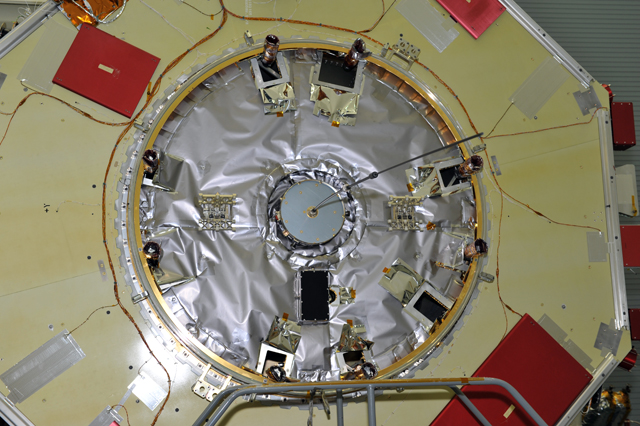
ADP was designed based on a proven deployable rigid boom design provided by ATK using long graphite coilable booms that are deployed from the thrust tube of the MMS spacecraft as close to the spin axis as possible. The distance from tip to tip will be on the order of 30.4 meters which is the maximum achievable length given the technical limitations, also looking at the preservation of spacecraft stability.

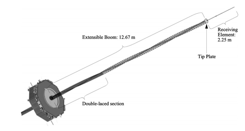
The rigid booms use a well-known design provided by ATK (now Orbital ATK) with each coilable boom being 12.67 meters in length carrying on its tip a second, smaller boom referred to as the receiving element. These booms have a 30.9-centimeter guard ring that is 2.6cm high and encircles the mounting plate at the end of the boom and smaller guard rings are installed on the outboard end of each coilable boom for shading. The 2.25-meter long secondary rigid booms are installed on the coiled boom and folded onto the top and bottom of the spacecraft. The small outer boom deploys soon after launch followed after the SDP deployment by the long 12.67m coiled boom.

The outer booms consist of a 90° base hinge, a 0.78m long by 1cm diameter tube, a 180° elbow hinge, a 0.43m long by 0.95cm diameter tube, a preamplifier 5.6cm long and 2.1cm in diameter and a 1-meter long 0.64cm diameter sensor. All booms are helically twisted by 60° every two meters so that the illuminated area remains constant with the spacecraft rotation which is critical given the influence of photoelectron currents on the measurement results.

Another important consideration was the symmetry between the top and bottom boom since the booms have to be mounted symmetric about the spacecraft’s electrostatic plane. Because the SDP wire booms are offset to the top side of the spacecraft, the lower ADP boom is recessed by 10cm into the spacecraft body to maintain a perfect symmetry.

The ADP extendable boom consist of a truss-like structure with three monolithic longerons running the entire length of the boom, held in place by graphite-composite battens (creating separation force between the longerons) and stainless steel wire rope diagonals (restricting the separation between longerons to create a rigid assembly).

In a deployed configuration, the battens are compressed and the ropes are under tension, creating a tensional integrity of the structure. The lower segment of the boom is double-laced with twice the number of battens and ropes to provide additional strength needed during spacecraft accelerations.

The booms are helically twisted by 60° every two meters to ensure the same surface area is exposed to the sun to limit the modulation of photoelectron generation near the receiving end. The entire ADP exterior is electrically isolated from the MMS spacecraft platform and connected to the Digital Signal Processor grounding. A shielded cable with five connectors runs the entire length of each longeron so that the critical signals can be wired redundantly. The signal interfaces are wired through a breakout board at the tip plate.

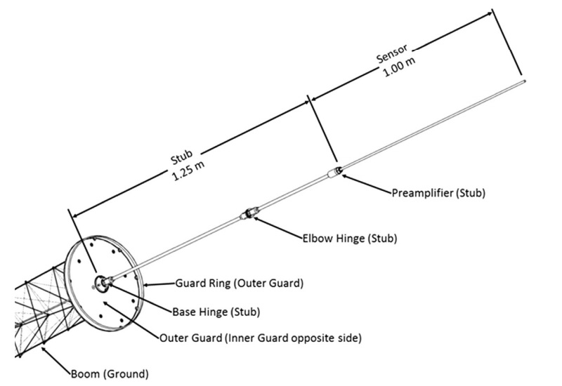
Atop the main ADP boom sits a disk-shaped tip plate with its two sides electrically isolated from the boom. The inner and outer surfaces are referred to as guards and carry a potential controlled by the main electronics of the instrument. The 30.9 centimeter guard ring has the same potential as the outer guard and shadows the tip plate to avoid photoelectron emissions towards the ADP sensor.

The lower 1.25-meter segment of the receiving element is known as the stub, it includes a 90° base hinge, a 0.78cm long 1cm diameter tube, a 180° elbow hinge and a 0.43 centimeter boom at 0.95cm diameter interfacing with the 5.6cm long and 2.1cm diameter preamplifier. The entire stub carries a separate potential and inside the tubes runs the electrical connection of the preamp, maintaining an axial symmetry. The outer surface of the stub is coated with DAG213 (graphite in an epoxy matrix) while the hinges use a coating of electroless nickel and co-deposited polytetrafluoroethylene. The outer housing of the preamp is connected to the stub and has the same electrical potential.

The preamp electronics are enclosed in a brass radiation shield connected to the preamp output via a resistor to reduce capacitive coupling with the preamp case which improves high frequency performance. Installed on the outboard end of the preamp is the one-meter long and 0.64cm diameter cylindrical sensor tube, directly interfacing with the preamp input. Bias current is supplied by the instrument electronics as is the +/-14V floating ground with a range from -100V to +40V to allow the spacecraft instruments to operate in a variety of chassis potential ranges.

In the stowed configuration, the extendable boom is coiled inside of a canister while the receiving end is folded on the base and elbow hinge and held in place by two launch latches. In flight, the latches are opened by high-output paraffin actuators pushing the release mechanism over center that causes the simultaneous release of the latch arms.

The tip latch releases first followed by the elbow latch and redundant springs in each hinge deliver the strain energy needed for the deployment of the receiving end. The hinge springs hold the hinges against a hard stop in the fully deployed configuration, preventing any flexing during routine spacecraft maneuvers.

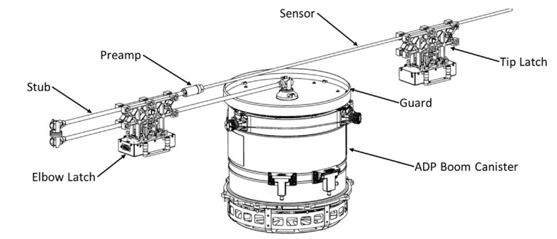
The ADP boom is coiled up in a 29cm diameter, 22cm high canister, secured within it using three spring-loaded pins. A frangibolt actuates the release mechanism, releasing a tensioned cable that pulls back the pins, allowing three kick over springs at the base of the boom to initiate the deployment.

The springs erect the lower segments of the longerons thus pushing the stack out of the canister so that the boom can then uncoil through the strain energy in the longerons. A damper controls the speed of the deployment through a lanyard attached to the tip of the boom. The ADP receiving ends are deployed first followed by the magnetometer and SDP booms until the ADP booms are released.

The ADP booms are designed to maintain an alignment within 0.18 degrees of the expected position to ensure data accuracy and no interference with other instrument data collection.

FIELDS Digital Signal Processor

 

The DSP of the FIELDS suite receives nine analog data signals from the Search Coil Magnetometers, the Axial Double Probes and the Spin Double Probes. The main task of the DSP is the conversion of the analog signals to a digital data stream that can be stored in the spacecraft memory and downlinked to Earth. Analog to Digital Conversion is completed by an Actel RTAX2000 Field Programmable Gate Array.

Two DSPs are installed in the Central Electronics Box of the MMS spacecraft, the primary unit is actively executing its tasks while the other remains unpowered to be activated in case of problems with the primary system. The signals arriving at DSP-A are routed directly to DSP-B regardless of which unit is the active one. Due to the high impedance on each DSP, the powered-off unit does not disturb the sensor signals that are processed. The grounds of the Boom Electronics Boards, the Axial Electronics Board and the Search Coil Magnetometer are connected directly through the DSP. The two DSPs are connected to analog ground via a common backplane.

The DSP is also in charge of data volume reduction using broad band filters, digital waveform filtering, spectral processing, burst memory and solitary structure detection. MMS normally operates in a survey mode where the instruments deliver continuous low-rate data throughout the orbit with the exception of certain period when passing through the regions of active reconnection during which high-cadence measurements will be made. Also, a burst mode is available to momentarily switch all or a subset of the instruments to high-time resolution measurements based on an event trigger.

FIELDS Central Electronics Box

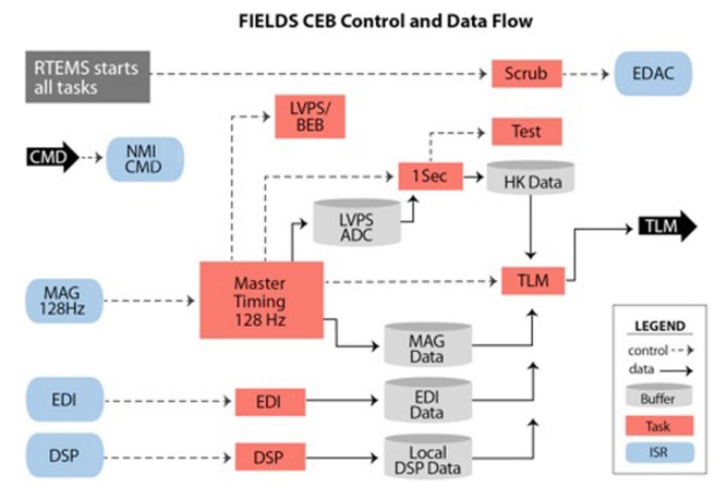
The CEB of the FIELDS Suite includes the Central Data Processing Unit for the Fields Package, the Digital Signal Processor for the Double Probes, the EDI controllers, magnetometer electronics and various electronics to control the timing of the instruments and condition telemetry and science data streams.

All magnetometer data from the Digital and Analog Fluxgate Magnetometer instruments is supplied via the AFG as a continuous stream of 128 vectors per second from both instruments. The CEB performs digital data filtering down to the commanded data rate. Also, CEB puts the data through onboard processing for internal coordinate system rotation for use by other onboard instruments in real time.

The EDI data is taken directly from the instrument controller that is in charge of processing to the commanded data rates and the same is done for data from the Digital Signal Processor which can complete all processing tasks by itself based on commands provided by the central spacecraft controllers. Some data delivered from DSP and EDI are used in the onboard algorithms that are in charge of burst mode triggers based on pre-set event thresholds. The CEB includes the Low Voltage Power Supply used to deliver electronics power to all FIELDS components and dedicated power supplies are produce the floating power required by the double probes.

Each of the Fields sensors can deliver data at different sampling rates as low as 0.5 samples per second for the magnetometers and double probes to as high as 262,144 samples per second for the electric and magnetic sensors when operating in burst mode. All DSP input channels are used to generate products over a 1024-sample time series to be sent as averaged frequency spectrums. Additional data streams conditioned by CEB include housekeeping and calibration data was well as timing products. DSP can deliver burst data on two High-Speed Burst Channels and also has an output of Solitary Wave Detector data.

All data from CEB is delivered to the Central Instrument Data Processor for storage and downlink to the ground. Due to the large volume of data collected in burst and high data rate modes, onboard processing is employed to select samples that show a promising structure.

CEB of FIELDS is also in charge of timing signal generation since all instruments within the suite are required to sample on the same synchronous time defined by an independent clock. The FIELDS clock runs asynchronously from to those in the Central Instrument Data Processing Unit and the rest of the spacecraft. Timing signals are generated through GPS as a Pulse Per Second signal that is distributed across the spacecraft with very high accuracy. Correlation data within the telemetry stream from FIELDS and known instrument characteristics are used to determine the absolute times of acquisition. Extensive calibration was completed to ensure an accurate inter-sensor timing.

Active Spacecraft Potential Control Device

To be able to measure low-energy ions and electrons, the electrical potential building up on the MMS spacecraft as it flies through the charged plasma has to be neutralized. Two Active Spacecraft Potential Control Devices are installed on each MMS spacecraft using indium ion beams to adjust the spacecraft potential. The indium beams generated by the ASPOC can have energies of 4 to 12 keV and current up to 70 microamps running in an antiparallel direction.

The ion generators are Liquid Metal Ion Sources that consist of a needle covered with indium and heated above the melting point of the metal at 156.6°C. Applying a sufficiently high electric potential between the emitter and the extractor electrode will lead to a change in the equilibrium between surface tension and electric field strength, forming a Taylor cone on the surface with a jet protruding from it.

Indium atoms are ionized at the edge of the jet and accelerated outward by the electric field. The expelled ions are then replenished by the hydrodynamic flow in the liquid metal.

Through feedback control, the system will keep the spacecraft potential at several volts positive. Each ASPOC consists of digital boards, low voltage and high voltage power supplies and two cylindrical emitters. Each emitter module has two ion sources driven by a common voltage supply connected via a cable harness routed outside the electronics box. During operation, only one ion source is active.

Ground Segment

The MMS Mission Operations Center is located at the Goddard Spaceflight Center and is responsible for spacecraft operations and telemetry analysis while the Flight Dynamics Operations Area, also at Goddard, completes orbit determination and maneuver development for formation-keeping and orbit adjustments. The Science Operations Center is situated at LASP and is in charge of instrument suite operations including commanding and instrument maintenance as well as science data processing, distribution and archiving. Instrument teams from each participating institution are responsible for data analysis and validation, instrument monitoring, observation requests and public distribution of science results.